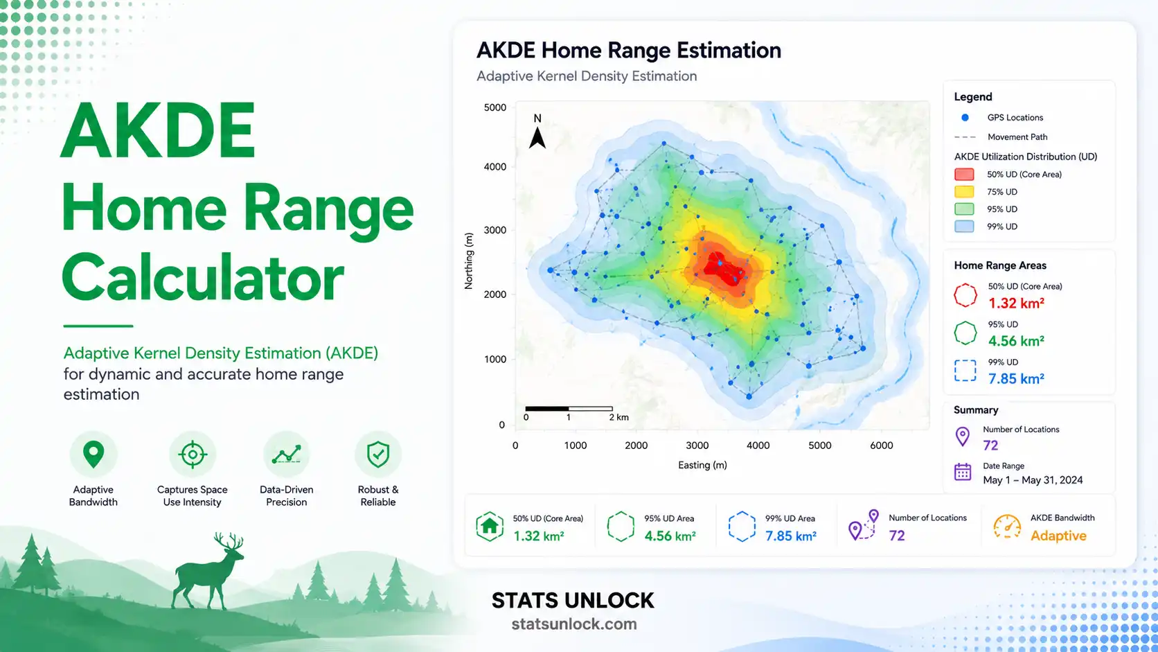
AKDE Home Range Calculator – Autocorrelated KDE Estimator

📍 Step 1 — Enter GPS Telemetry Data (Latitude & Longitude)

Latitudes (decimal degrees)

Comma- or newline-separated. WGS84 decimal degrees. Default sample: Yellowstone gray wolf (USA).

Longitudes (decimal degrees)

Must match the number of latitude values exactly.

Fix interval (hours, optional)

Time between consecutive GPS fixes. Used to estimate autocorrelation timescale.

Load a sample dataset

Upload CSV or Excel file

Supports .csv, .txt, .xlsx, .xls — choose latitude & longitude columns after upload.

Latitude Longitude Actions

0 valid fixes entered

⚙️ Step 2 — Configure Analysis

Group / Individual Name (editable)

Area unit

Primary contour (%)

Kernel function

📊 Results — Summary

📈 Four Visualizations of the Home Range

Each plot illuminates a different facet of the AKDE result — spatial distribution, utilization density, autocorrelation structure, and movement path.

🗺️ 1. GPS Fixes & Home Range Contours

95%, 90%, 75% & 50% contour ellipses with all telemetry points

🌡️ 2. Utilization Distribution (UD)

Kernel density surface — heat-style hexbin intensity

📉 3. Variogram (Autocorrelation)

Semivariance vs time-lag → estimates τ

🚶 4. Movement Trajectory

Time-ordered path coloured by sequence

AKDE Home Range Equation

The autocorrelated kernel density estimate of the utilization distribution f̂(x) is:

f̂(x) = 1 N_eff · h² ∑_i=1^N K ( x − x_i h )

h = σ̂ · N_eff^−1/6 · √2 N_eff = N · Δt Δt + 2τ

A_p = π · k_p · (σ̂² + h²) · N_eff + 1 N_eff k_p = −2 · ln(1 − p/100)

f̂(x): Estimated utilization distribution at location x
x_i: Observed GPS fix i (latitude/longitude projected to UTM metres)
K: Kernel function (Gaussian or Epanechnikov)
h: Bandwidth — automatically chosen via Gaussian-reference plug-in scaled by N_eff
σ̂: Pooled standard deviation of positions (proxy for spatial spread)
N: Raw number of GPS fixes
N_eff: Effective sample size, corrected for autocorrelation
Δt: Fix interval (time between consecutive GPS records)
τ: Autocorrelation timescale — time for position autocorrelation to decay
A_p: Area of the p% utilization contour (computed for p = 95, 90, 75, 50)
k_p: Chi-square scaling for the bivariate Gaussian — k₉₅ = 5.99, k₉₀ = 4.61, k₇₅ = 2.77, k₅₀ = 1.39
∑: Sum across all N fixes

📋 Copy significance statement

🧭 Detailed Interpretation of Results

✍️ How to Write Your Results in Research (5 Examples)

Five ready-to-use reporting templates, each auto-filled with your AKDE results — copy any one to use directly in your manuscript, thesis, or report.

🪧 Research Poster Panel — Visual Science Communication

📐 Poster Design Specifications

Typography: Title 72–96 pt; section headings 36–48 pt; body 24–32 pt; references 14–18 pt; recommended font pairing: DM Sans (body) + Inter / Roboto Slab (headings).

Colour palette: Background #ffffff or #f7fafc; accents in the AKDE green (#0e7c5a); use blue (#2563eb) for movement-path graphics and magenta (#db2777) for the UD heat surface.

Poster sizes: A0 (841×1189 mm), A1 (594×841 mm), or 36×48 in. (USA ESA / TWS standard).

Print resolution: Vector text + 300 dpi raster images; export PDF/X-1a for commercial print.

Software: Adobe Illustrator, Inkscape (free), Affinity Publisher, PowerPoint, or LaTeX (a0poster / tikzposter).

🎯 Conclusion

📌 What Was Found

🌍 Ecological Significance

🌿 Conservation & Management Implications

🔭 Next Steps & Methodological Guidance

🎯 When to Use AKDE

Use this decision checklist to confirm AKDE is the right home range estimator for your dataset.

✅ AKDE is appropriate when:

✓ You have ≥ 30 GPS fixes for one individual

✓ Fixes are regular in time (e.g. every 1–4 hours)

✓ The animal is range-resident (not migrating)

✓ You want statistically honest 95%, 90%, 75%, and 50% contours

✓ Fix rate is fast enough to capture autocorrelation

✓ You need to compare home ranges across animals

⚠️ AKDE is NOT appropriate when:

✗ Fewer than 30 fixes (too few for τ estimation)

✗ Animal is dispersing or migrating

✗ Mark-recapture or census data (use MCP instead)

✗ Multiple animals pooled (estimate each separately)

🌎 Real-world USA examples:

Yellowstone gray wolves — 4-hour GPS collars; AKDE produces 600–1500 km² ranges vs ~300 km² from KDE.
Florida panthers — Hourly fixes; AKDE corrects for fine-scale autocorrelation in dense palmetto habitat.
Greater Yellowstone grizzly bears — Mixed seasonal residency; AKDE preferred over MCP for seasonal range overlap.
Mojave desert tortoises — Slow-moving, long τ; AKDE essential to avoid effective-N inflation.

📖 How to Use This Tool — Step-by-Step Guide

STEP 1 — Enter your data. Use the Paste/Type tab for comma-separated latitude and longitude. Upload tab supports CSV/Excel with column picker. Manual tab lets you build a small grid.
STEP 2 — Pick a sample dataset (optional) from the dropdown to preview a realistic USA telemetry scenario.
STEP 3 — Configure analysis settings. Set the group/individual name, area unit (km² is standard for wildlife studies), contour percentage (95% is the default home range), and kernel function (Gaussian recommended).
STEP 4 — Click "Run AKDE Analysis." The tool projects latitudes/longitudes to UTM-style metres, computes the autocorrelation timescale τ from a variogram, derives the effective sample size, and integrates the bivariate kernel surface to yield 95%, 90%, 75%, and 50% contour areas.
STEP 5 — Read the summary cards. Green = high reliability, amber = moderate, red = under-sampled.
STEP 6 — Read the full results table. Each row explains a quantity (area, bandwidth, τ, N_eff, projected metres).
STEP 7 — Examine all four visualizations. Spatial scatter, UD heatmap, variogram, trajectory.
STEP 8 — Read the detailed interpretation. Useful for thesis chapters, park-management briefs, and journal discussion sections.
STEP 9 — Copy a reporting example. Five ready-to-use formats from journal style to plain-language brief.
STEP 10 — Export your results. Download as .txt (Doc) or print-ready PDF.

🔬 Technical Notes — Formula Derivation, Assumptions, Limitations

Bandwidth derivation. The Gaussian-reference plug-in bandwidth h = σ̂ · N_eff^−1/6 · √2 is Silverman's (1986) rule generalised to bivariate Gaussian data; the multiplier √2 yields an isotropic 2-D bandwidth from the 1-D form.

Autocorrelation timescale τ. Estimated from the empirical variogram of step distances. The semivariance γ(h) approaches its asymptote (sill) at a time-lag equal to ≈ τ. We fit a non-linear least-squares Ornstein-Uhlenbeck curve to the binned variogram.

Effective sample size N_eff. Derived from Bartlett's (1946) correction: N_eff = N · Δt / (Δt + 2τ). Heavy autocorrelation (τ ≫ Δt) collapses N_eff well below N.

Assumptions. (1) Range residency — animal does not migrate or disperse during the sampling window. (2) Stationarity — the underlying movement process is time-invariant. (3) Ornstein-Uhlenbeck or OUF movement model adequately approximates the data. (4) GPS error is small relative to home range diameter.

Limitations. Plug-in AKDE gives a point estimate but no formal confidence interval — use the ctmm R package (Calabrese et al. 2016) for bootstrap CIs and AIC-based model selection. Coarse fix rates (e.g. one fix per day) may miss the autocorrelation peak and bias τ low.

❓ Frequently Asked Questions

Q1. What is AKDE home range estimation and when should I use it?

Autocorrelated Kernel Density Estimation (AKDE), developed by Fleming et al. (2015), is a movement-model-based home range estimator that explicitly accounts for the autocorrelation present in modern GPS telemetry data. Use AKDE whenever consecutive locations are correlated in time — which is almost always the case with fix rates faster than one fix per day. Conventional KDE assumes independence and severely underestimates home range area; AKDE corrects this bias.

Q2. What data do I need to calculate AKDE?

You need GPS relocation data for a single individual: latitude, longitude, and (ideally) the fix interval in hours. A minimum of 30 fixes is required; 50–100 is recommended for reliable τ estimation; 200+ is excellent. Regular sampling intervals give the best autocorrelation estimates. The tool accepts comma-separated values, CSV uploads, Excel files, or manual entry.

Q3. What does a high vs low AKDE home range area mean ecologically?

A larger home range indicates an animal moving over greater distances — often associated with low resource density, large-bodied species, carnivores, or open habitat. A small home range suggests high site fidelity, abundant resources, or constrained dispersal. For context: a Yellowstone wolf pack typically uses 200–1500 km², a black bear 5–250 km², a red fox 1–10 km², and a desert tortoise less than 1 km². Always interpret area alongside τ — long τ suggests slow movement, short τ rapid movement.

Q4. How does AKDE differ from conventional KDE or Minimum Convex Polygon (MCP)?

MCP draws the smallest convex polygon enclosing all fixes — simple but very sensitive to outliers. Conventional KDE assumes independent fixes and produces smooth density contours but underestimates area when fixes are autocorrelated. AKDE corrects KDE by computing an effective sample size from the autocorrelation timescale, producing a larger, statistically honest estimate. Calabrese et al. (2016) demonstrated AKDE outperforms both for typical GPS datasets.

Q5. What are the assumptions and limitations of AKDE?

Assumptions: (1) range residency — no migration or dispersal during the sampling period; (2) stationarity — movement process does not change over time; (3) an OU or OUF movement model approximates the animal's behaviour; (4) GPS error is small relative to the range diameter. Limitations: plug-in estimates lack formal confidence intervals; coarse fix rates may miss autocorrelation; pooled-individual analysis is not recommended (estimate each animal separately).

Q6. How much sampling effort do I need for AKDE to be reliable?

Minimum 30 fixes; reliable from 50; excellent at 200+. The key metric is N_eff — the effective sample size after correcting for autocorrelation. Aim for N_eff ≥ 25–50 for honest 95% contours and ≥ 50–100 for honest 50% (core area) contours. Heavy autocorrelation (long τ) collapses N_eff, so faster fix rates do not always help — they may need to be balanced with longer tracking durations.

Q7. Can I compare AKDE home ranges between animals or sites?

Yes, provided sampling effort (number of fixes, fix interval, study duration) is standardized. Always report N, N_eff, τ, and Δt alongside the area. For formal hypothesis tests use the ctmm R package which provides Bhattacharyya overlap coefficients, AKDE-CI overlap, and bootstrap confidence intervals.

Q8. How do I report AKDE results in an ecology journal or conservation report?

Report: (a) the 95% home range area with units; (b) the 50% core area; (c) sample size N and effective sample size N_eff; (d) the autocorrelation timescale τ; (e) the fix interval Δt; (f) the kernel function used; and (g) citations to Fleming et al. (2015) and Calabrese et al. (2016). See Section 2.7 for five ready-to-use templates (journal, thesis, policy brief, conference abstract, monitoring report).

Q9. Can I use this calculator for published research or a university thesis?

Yes for educational use, exploratory analysis, and figure prototyping. For peer-reviewed publication we recommend cross-validating with the ctmm R package which provides AIC-based movement model selection (IID, OU, OUF), bootstrap confidence intervals, and Bhattacharyya overlap coefficients. Cite this tool as: "Stats Unlock (2026). AKDE Home Range Calculator. Retrieved from https://statsunlock.com."

Q10. My home range estimate seems unexpectedly large or small — what might be wrong?

Common issues: (a) Mixed-up latitude/longitude columns (swap them and re-run). (b) Dispersal or migration during the sampling window (subset to a residency period). (c) GPS error spikes — check for fixes hundreds of km from the cluster. (d) Coarse fix rate masking τ — try a faster-fix dataset. (e) Two animals' data accidentally pooled. (f) Wrong area unit. Always inspect the Trajectory plot (Chart 4) for obvious outliers before trusting the area estimate.

📚 References

Foundational and methodological sources for autocorrelated kernel density estimation, the ctmm framework (Fleming et al. 2015; Calabrese et al. 2016), and comparison with alternative home range estimators.

Fleming, C. H., Fagan, W. F., Mueller, T., Olson, K. A., Leimgruber, P., & Calabrese, J. M. (2015). Rigorous home range estimation with movement data: A new autocorrelated kernel density estimator. Ecology, 96(5), 1182–1188. https://doi.org/10.1890/14-2010.1
Calabrese, J. M., Fleming, C. H., & Gurarie, E. (2016). ctmm: an R package for analyzing animal relocation data as a continuous-time stochastic process. Methods in Ecology and Evolution, 7(9), 1124–1132. https://doi.org/10.1111/2041-210X.12559
Worton, B. J. (1989). Kernel methods for estimating the utilization distribution in home-range studies. Ecology, 70(1), 164–168. https://doi.org/10.2307/1938423
Silverman, B. W. (1986). Density Estimation for Statistics and Data Analysis. Chapman & Hall/CRC. https://doi.org/10.1201/9781315140919
Fleming, C. H., Calabrese, J. M., Mueller, T., Olson, K. A., Leimgruber, P., & Fagan, W. F. (2014). From fine-scale foraging to home ranges: A semivariance approach to identifying movement modes across spatiotemporal scales. The American Naturalist, 183(5), E154–E167. https://doi.org/10.1086/675504
Noonan, M. J., Tucker, M. A., Fleming, C. H., et al. (2019). A comprehensive analysis of autocorrelation and bias in home range estimation. Ecological Monographs, 89(2), e01344. https://doi.org/10.1002/ecm.1344
Seaman, D. E., & Powell, R. A. (1996). An evaluation of the accuracy of kernel density estimators for home range analysis. Ecology, 77(7), 2075–2085. https://doi.org/10.2307/2265701
Burt, W. H. (1943). Territoriality and home range concepts as applied to mammals. Journal of Mammalogy, 24(3), 346–352. https://doi.org/10.2307/1374834
Kie, J. G., Matthiopoulos, J., Fieberg, J., Powell, R. A., Cagnacci, F., Mitchell, M. S., Gaillard, J.-M., & Moorcroft, P. R. (2010). The home-range concept: Are traditional estimators still relevant with modern telemetry technology? Philosophical Transactions of the Royal Society B, 365(1550), 2221–2231. https://doi.org/10.1098/rstb.2010.0093
Gurarie, E., Fleming, C. H., Fagan, W. F., Laidre, K. L., Hernández-Pliego, J., & Ovaskainen, O. (2017). Correlated velocity models as a fundamental unit of animal movement: Synthesis and applications. Movement Ecology, 5, 13. https://doi.org/10.1186/s40462-017-0103-3
Signer, J., Fieberg, J., & Avgar, T. (2019). Animal Movement Tools (amt): R package for managing tracking data and conducting habitat selection analyses. Ecology and Evolution, 9(2), 880–890. https://doi.org/10.1002/ece3.4823
Powell, R. A., & Mitchell, M. S. (2012). What is a home range? Journal of Mammalogy, 93(4), 948–958. https://doi.org/10.1644/11-MAMM-S-177.1
Cagnacci, F., Boitani, L., Powell, R. A., & Boyce, M. S. (2010). Animal ecology meets GPS-based radiotelemetry: A perfect storm of opportunities and challenges. Philosophical Transactions of the Royal Society B, 365(1550), 2157–2162. https://doi.org/10.1098/rstb.2010.0107
Smouse, P. E., Focardi, S., Moorcroft, P. R., Kie, J. G., Forester, J. D., & Morales, J. M. (2010). Stochastic modelling of animal movement. Philosophical Transactions of the Royal Society B, 365(1550), 2201–2211. https://doi.org/10.1098/rstb.2010.0078
R Core Team. (2024). R: A language and environment for statistical computing. R Foundation for Statistical Computing. https://www.R-project.org/