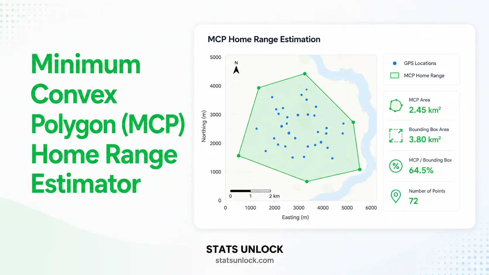
Minimum Convex Polygon (MCP) Home Range Estimator

📥 1. Enter Your GPS Location Data

Latitudes (decimal degrees) — comma-separated

Decimal degrees (N/S). One value per comma. Sample: 52, 48, 55, 61, 47, ... style format supported.

Longitudes (decimal degrees) — comma-separated

Decimal degrees (W = negative, E = positive). Must have the same number of values as the latitudes.

Upload CSV or Excel file (.csv, .txt, .xlsx, .xls)

Supports .csv, .txt, .xlsx, .xls. Headers auto-detected. After upload, choose the latitude and longitude columns below.

Click "Add Point" in the Column Entry mode above for structured point-by-point input. The manual table below is a quick spreadsheet alternative.

#	Latitude	Longitude

⚙️ 2. Configuration

Study Area / Site Name (optional)

Group / Individual Name

Area Unit

Isopleth Percentage

Sample Dataset

📊 3. Results

📈 Four Visualizations of the Home Range

Spatial polygon, distance distribution, isopleth comparison, and sample-size adequacy curve.

🗺️ MCP Polygon Map (GPS Points)

📏 Distance from Centroid (Histogram)

📊 MCP Area by Isopleth Percentage

📈 Cumulative Area Curve (Sample-Size Adequacy)

🌐 Empirical CDF — Distance from Centroid

🧭 Nearest-Neighbour Distance Distribution

📐 Movement & Spread Statistics

🔬 Shape, Density & Confidence Interval

Minimum Convex Polygon (MCP) Area Formula

MCP area is computed from the convex hull of n GPS location points using the shoelace formula:

Area = ½ × | Σ_i=1ⁿ (x_i · y_i+1 − x_i+1 · y_i) |

Area: MCP polygon area (m², converted to ha or km²)
n: number of vertices of the convex hull
x_i, y_i: projected coordinates (in meters) of the i-th hull vertex
Σ: sum over all hull vertices, cyclically (i+1 wraps to 1)
95% MCP: identical formula applied to the 95% of points closest to the arithmetic centroid (5% outliers dropped)
Projection: Equirectangular (mean-latitude scaled) — accurate for <500 km extent

Detailed Results

📎 Copy Summary to Clipboard

📖 How to Use This Tool — Step-by-Step Guide

Enter your GPS data. Paste latitudes and longitudes (decimal degrees, comma-separated), upload a CSV/Excel file, or fill the manual table. Example for a grizzly bear in Yellowstone, USA: paste lat values like 44.4280, 44.4351, 44.4198, ... and matching longitudes.
Choose a sample dataset. Five real-world USA wildlife examples are provided (grizzly bear, gray wolf, mountain lion, white-tailed deer, mule deer). Dataset 1 is pre-loaded.
Configure the analysis. Set the area unit (hectares, km², m²), choose the isopleth percentage (default: both 100% and 95% MCP). Optionally enter a Study Area Name (e.g., "Yellowstone National Park") and a Group / Individual Name (e.g., "Female Grizzly #07").
Click "Calculate MCP Home Range". The tool computes the convex hull, area, perimeter, centroid, and four visualization plots.
Read the summary cards. Green = small/stable home range typical for the species. Amber = moderate range. Red = unusually large range (possible dispersal or sampling artefact).
Inspect the four plots. (1) Spatial polygon map shows the actual home range outline; (2) Distance-from-centroid histogram reveals how spatially clustered the points are; (3) Bar chart compares 100% vs 95% MCP area; (4) Cumulative area curve shows whether your sample size is adequate (curve should plateau).
Read the Detailed Interpretation. The auto-generated paragraphs explain what your MCP area means ecologically, with site name substituted throughout.
Copy a reporting example. Choose the journal, thesis, policy, abstract, or monitoring format that matches your audience.
Use the Research Poster panel. The poster section auto-fills with your results in conference-ready layout.
Export your results. Download as Word-compatible .txt for reports, or PDF for printing and archiving.

❓ Frequently Asked Questions

Q1. What is a Minimum Convex Polygon (MCP) home range estimator and when should I use it?

The Minimum Convex Polygon (MCP) is the smallest convex polygon enclosing every GPS or telemetry location of an animal. It is the oldest, most widely reported home range estimator in wildlife ecology, introduced by Mohr (1947). Use it when you need a simple, reproducible perimeter, when comparing to historical studies that used MCP, or as a baseline alongside kernel density estimators.

Q2. What data do I need to calculate MCP home range?

You need a list of GPS locations as paired latitude and longitude values (decimal degrees). At minimum 5 points are required to form a polygon, but 30 or more independent locations are recommended for a reliable estimate. The Paste/Type tab accepts comma-separated values; the Upload tab handles CSV and Excel files; the Manual Table accepts row-by-row entry.

Q3. What does a large vs small MCP home range mean ecologically?

Home range size reflects body size, diet, habitat productivity, and social system. Large mammals (bears, wolves) commonly have ranges of 100–10,000+ km²; meso-carnivores (foxes, lynx) 10–100 km²; ungulates (deer, elk) 1–50 km². An unusually large value may indicate dispersal, low resource availability, or extreme outlier locations. Compare against published values for the species.

Q4. How does MCP differ from kernel density estimation (KDE)?

MCP gives a single bounded area — the convex hull of the points. KDE produces a continuous utilization distribution (UD) and lets you compute core areas (50% UD) and full home range (95% UD). MCP overestimates area by including unused habitat inside the polygon; KDE provides a more realistic intensity surface. Most modern studies report both for comparison with historical and recent literature.

Q5. What are the assumptions and limitations of MCP?

MCP assumes the animal uses the entire enclosed area uniformly (rarely true), and is highly sensitive to outlier points — a single dispersal excursion can double the area. It does not account for unused habitat, barriers (rivers, roads), or detection probability. The 95% MCP option mitigates the outlier problem by dropping the 5% of points farthest from the arithmetic centroid.

Q6. How many GPS points do I need for a reliable MCP home range?

Minimum 30 independent fixes. Many studies recommend 50+. Use the Cumulative Area Curve (Plot 4) to assess adequacy — when the curve plateaus, additional points are not adding new range, and your estimate is stable. If the curve is still rising at the end, your home range is likely under-estimated.

Q7. Can I compare MCP home range values between individuals or seasons?

Yes, but only if sampling effort and duration are standardised. Differences in fix rate, tracking duration, or season strongly affect MCP area. Always compare 95% MCP rather than 100% MCP, report the sample size, and consider seasonal subsets. For rigorous comparison, use a bootstrap or permutation test on equal-effort subsets.

Q8. How do I report MCP home range in a wildlife journal?

Always include: the percent isopleth (e.g., "95% MCP"), the area with units (e.g., "1,247 ha" or "12.47 km²"), the number of locations (n), the sampling period (e.g., "1 May – 31 October 2024"), the projection / CRS used, and a citation to Mohr (1947). See the five reporting examples in Section 4 above for templates by audience.

Q9. Can I use this calculator for published research or a thesis?

This tool is designed for educational use, classroom exercises, and exploratory analysis. For peer-reviewed publication or thesis work, verify your results in R using the adehabitatHR package (function mcp()) or in Python with movingpandas, which support proper coordinate projection and handle large datasets. Cite this tool as: "Stats Unlock. (2026). Minimum Convex Polygon Home Range Estimator. Retrieved from https://statsunlock.com".

Q10. My MCP area seems unexpectedly large or small — what might be wrong?

Common causes: (1) one or two outlier GPS fixes from a long-distance excursion — try the 95% MCP option; (2) latitude/longitude columns swapped — check that latitudes range −90 to 90 and longitudes −180 to 180; (3) coordinates in degrees-minutes-seconds rather than decimal degrees; (4) too few points (under 30) producing an unstable estimate; (5) the cumulative area curve has not plateaued — add more tracking days.

📚 References

Foundational and methodological sources for the MCP method, sample-size adequacy, alternative estimators, and the convex-hull algorithm used by this tool.

Mohr, C. O. (1947). Table of equivalent populations of North American small mammals. American Midland Naturalist, 37(1), 223–249. https://doi.org/10.2307/2421652
Burt, W. H. (1943). Territoriality and home range concepts as applied to mammals. Journal of Mammalogy, 24(3), 346–352. https://doi.org/10.2307/1374834
Worton, B. J. (1989). Kernel methods for estimating the utilization distribution in home-range studies. Ecology, 70(1), 164–168. https://doi.org/10.2307/1938423
White, G. C., & Garrott, R. A. (1990). Analysis of wildlife radio-tracking data. Academic Press.
Powell, R. A., & Mitchell, M. S. (2012). What is a home range? Journal of Mammalogy, 93(4), 948–958. https://doi.org/10.1644/11-MAMM-S-177.1
Laver, P. N., & Kelly, M. J. (2008). A critical review of home range studies. Journal of Wildlife Management, 72(1), 290–298. https://doi.org/10.2193/2005-589
Calenge, C. (2006). The package "adehabitat" for the R software: A tool for the analysis of space and habitat use by animals. Ecological Modelling, 197(3–4), 516–519. https://doi.org/10.1016/j.ecolmodel.2006.03.017
Seaman, D. E., Millspaugh, J. J., Kernohan, B. J., Brundige, G. C., Raedeke, K. J., & Gitzen, R. A. (1999). Effects of sample size on kernel home range estimates. Journal of Wildlife Management, 63(2), 739–747. https://doi.org/10.2307/3802664
Getz, W. M., & Wilmers, C. C. (2004). A local nearest-neighbor convex-hull construction of home ranges and utilization distributions. Ecography, 27(4), 489–505. https://doi.org/10.1111/j.0906-7590.2004.03835.x
Kie, J. G., Matthiopoulos, J., Fieberg, J., Powell, R. A., Cagnacci, F., Mitchell, M. S., Gaillard, J.-M., & Moorcroft, P. R. (2010). The home-range concept: Are traditional estimators still relevant with modern telemetry technology? Philosophical Transactions of the Royal Society B, 365(1550), 2221–2231. https://doi.org/10.1098/rstb.2010.0093
Fieberg, J., & Börger, L. (2012). Could you please phrase "home range" as a question? Journal of Mammalogy, 93(4), 890–902. https://doi.org/10.1644/11-MAMM-S-172.1
Signer, J., Fieberg, J., & Avgar, T. (2019). Animal movement tools (amt): R package for managing tracking data and conducting habitat selection analyses. Ecology and Evolution, 9(2), 880–890. https://doi.org/10.1002/ece3.4823
Walter, W. D., Onorato, D. P., & Fischer, J. W. (2015). Is there a single best estimator? Selection of home range estimators using area-under-the-curve. Movement Ecology, 3(1), 10. https://doi.org/10.1186/s40462-015-0039-4
Andrew, A. M. (1979). Another efficient algorithm for convex hulls in two dimensions. Information Processing Letters, 9(5), 216–219. https://doi.org/10.1016/0020-0190(79)90072-3
R Core Team. (2024). R: A language and environment for statistical computing. R Foundation for Statistical Computing. https://www.R-project.org/