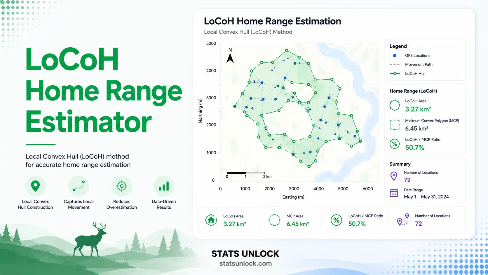
Local Convex Hull (LoCoH) Home Range Estimator
A free online LoCoH home range estimator for wildlife biologists. Convert GPS or radio-telemetry coordinates into a publication-ready local convex hull home range with core areas, isopleth analysis, and interpretation.
📥 1 · Input GPS Coordinates
Enter paired latitude and longitude relocations from a single individual. Default sample data uses a USA white-tailed deer GPS track.
0 fixes parsed
Supports .csv, .txt, .xlsx, .xls — headers auto-detected. Two numeric columns required (latitude + longitude).
Enter latitude / longitude pairs row by row.
0 fixes entered
⚙️ 2 · Analysis Configuration
Editable. Used throughout report.
k: integer neighbors · a: distance sum (m) · r: radius (m)
All four isopleths (95 / 90 / 75 / 50) are reported together.
📊 Results Summary
LoCoH (Local Convex Hull) Formula
The LoCoH home range is the union of local convex hulls built around each relocation point:
where Hi = ConvexHull({Pi} ∪ Ni),
Areaiso = ⋃ Hi sorted ascending by area until ∑Area ≥ (iso% × Total)
- Pi: i-th relocation point (lat, lon)
- Ni: neighbourhood around Pi — k nearest neighbors (k-LoCoH), points within radius r (r-LoCoH), or adaptive set with Σd ≤ a (a-LoCoH)
- Hi: local convex hull from {Pi} ∪ Ni
- iso%: isopleth level — 95% is the home range, 50% is the core area
- UD: utilization distribution — the merged polygon of selected hulls
📋 Full Results Table
| Statistic | Value | Description |
|---|
📈 Four Colorful Visualizations
① Relocations + Nested 95 / 90 / 75 / 50% Isopleths
② Cumulative Isopleth Curve (50/75/90/95 marked)
③ Hull Area Distribution
④ Nearest-Neighbor Distance Histogram
🔬 Detailed Interpretation of Results
✍️ How to Write Your Results in Research
🪧 Research Poster Panel
🔍 Conclusion
▶ Run the analysis above to generate a personalized conclusion for your dataset.
🧮 Technical Notes
Formula derivation, assumptions, and limitations
Extended derivation. The Local Convex Hull (LoCoH) family was developed by Getz & Wilmers (2004) and refined by Getz et al. (2007). For each fix Pi with n relocations, a neighbourhood Ni is built using one of three rules:
- k-LoCoH: Ni = the (k − 1) Euclidean-nearest neighbors of Pi.
- r-LoCoH: Ni = all points within radius r of Pi.
- a-LoCoH: Ni = the largest set whose summed distances from Pi remain ≤ a.
A convex hull Hi = ConvexHull({Pi} ∪ Ni) is constructed for every fix using the Andrew monotone chain algorithm. Hulls are sorted in ascending area, then merged sequentially until the cumulative area reaches the chosen isopleth percent. The 95% isopleth is the home range; the 50% isopleth is the core area.
Assumptions. (1) Fixes are independent samples of space use. (2) The animal's range is approximately stationary during the sampling window. (3) The chosen parameter (k, a, or r) is appropriate for the local point density. (4) Coordinates are projected on a metric coordinate system before area computation — this tool projects WGS84 to a local meter grid at the centroid latitude.
Limitations. LoCoH can fragment ranges if k is too small; it can grossly over-estimate if k is too large (similar to MCP). Always plot the area-vs-k inflection curve and choose k near the elbow. LoCoH cannot, by itself, distinguish habitat selection or seasonal range shifts — pair with resource selection or step-selection analyses.
🎯 When to Use LoCoH
Decision checklist, examples, and related metrics
Decision Checklist
- You have at least 30 GPS or VHF relocations from one individual
- Your study area has hard boundaries (cliffs, water, roads) that MCP would over-fly
- You want a non-parametric, distribution-free home range estimator
- You need a method that converges to the true range with more data
- Do NOT use if you have fewer than 30 fixes — use MCP with caution instead
- Do NOT use if your fixes are extremely autocorrelated (sub-minute fix rate on a stationary animal)
Real-world examples (USA)
- Wildlife monitoring: Yellowstone wolf packs — LoCoH home ranges around den sites with multiple river crossings.
- Game management: Wisconsin white-tailed deer winter yard fidelity, where MCP would include unused agricultural fields.
- Predator ecology: Florida panther daily ranges with hard barriers from interstate highways.
- Avian telemetry: Chesapeake Bay bald eagle foraging ranges that exclude open water the bird never used.
Related metrics — when to pick which:
- Need a quick, classical estimate → MCP (Minimum Convex Polygon)
- Need a smooth probability surface → KDE (Kernel Density Estimation)
- Need an adaptive, sample-size-robust polygon → LoCoH (this tool)
- Need to compare ranges across treatments → run all three and report jointly
📘 How to Use This Tool — Step-by-Step
10-step worked example
- Enter your data. Paste comma-separated latitudes and longitudes, upload a CSV/Excel from your collar manufacturer, or type rows manually.
- Choose a sample dataset. Five USA wildlife datasets are pre-loaded; Deer #07 — Yellowstone NP is the default.
- Set the group/individual name. The name flows into all reports, citations, and the conclusion automatically.
- Pick the LoCoH method. a-LoCoH is recommended for most field studies because it adapts to point density.
- Set the parameter (k, a, or r). For k-LoCoH a good starting point is √n where n is your number of fixes.
- Choose the isopleth percent. 95% = home range, 50% = core area. Most papers report both.
- Click Calculate. The tool projects WGS84 to meters, builds local hulls, and merges them.
- Read the summary cards. Green = ample sample size and stable estimate; amber = borderline; red = under-sampled.
- Examine the four charts. Look at the isopleth curve elbow — that is your defensible parameter choice.
- Export. Download the .txt for sharing, the PDF for archiving, and copy the journal-style template into your manuscript.
❓ Frequently Asked Questions
Q1. What is the LoCoH home range estimator and when should I use it?
The Local Convex Hull (LoCoH) method is a non-parametric home range estimator that builds small convex hulls around clusters of relocations and merges them into one polygon. Use it whenever your study site contains unused space — water bodies, cliffs, highways, or vacant agricultural fields — that simpler methods such as Minimum Convex Polygon would falsely include. It is the recommended estimator for GPS-collared mammals and tagged raptors in heterogeneous landscapes.
Q2. What data do I need to calculate a LoCoH home range?
You need paired latitude and longitude relocations from a single individual, ideally in WGS84 decimal degrees. A minimum of 30 fixes is required to fit any LoCoH model; 100 or more fixes spread across the study period produces stable, publication-ready home ranges. The Paste tab works well for short tracks; Upload is the fastest path for full collar exports.
Q3. What does the 95% LoCoH isopleth mean ecologically?
The 95% isopleth defines the boundary that contains 95% of the merged local hulls and is the conventional home range. The 50% isopleth is the core area — the smaller polygon where the animal spends roughly half of its time. Areas above 95% are usually treated as transit or exploratory movements.
Q4. How does LoCoH differ from MCP and kernel density estimators?
MCP wraps one convex polygon around every fix and typically over-estimates the range because it includes unused space. KDE smooths a probability surface and may extend beyond points the animal ever visited. LoCoH respects hard boundaries and converges to the true range as sample size grows, making it the most defensible non-parametric estimator for fragmented habitats.
Q5. What are the assumptions and limitations of LoCoH?
Assumptions: relocations are independent samples of space use; the animal's range is stationary during the sampling window; and the parameter k, a, or r is appropriate for local point density. Limitations: very small k causes range fragmentation; very large k drifts toward MCP. Always plot the area-vs-parameter curve and pick the elbow.
Q6. How many GPS fixes do I need for a reliable LoCoH estimate?
30 fixes is the absolute minimum for a preliminary estimate. Most wildlife journals expect 100 or more fixes per individual, distributed across diel cycles and seasons. Below 30 fixes you should report area with caution and treat the polygon as exploratory.
Q7. Can I compare LoCoH home ranges between individuals or seasons?
Yes, but you must standardize fix rate, sample size, isopleth percent, and the LoCoH method (k, a, or r) across the comparison. Reporting different isopleths or different k values across individuals makes the comparison invalid. A bootstrap with random thinning is the cleanest way to confirm differences.
Q8. How do I report LoCoH home range in a wildlife journal?
State the method (k-, a-, or r-LoCoH), parameter value, number of fixes, isopleth percent, area in hectares or square kilometers, and the original citation (Getz et al., 2007). Always pair the 95% home range with the 50% core area. The reporting templates on this page produce all of this automatically.
Q9. Can I use this LoCoH calculator for published research?
This tool is intended for teaching, exploratory analysis, and reproducible classroom workflows. For peer-reviewed publication verify results with adehabitatHR or T-LoCoH in R and report exactly the parameter choices you used. Cite this tool as: STATS UNLOCK (2025). LoCoH Home Range Estimator. https://statsunlock.com/locoh-home-range-estimator.
Q10. My LoCoH home range looks wrong — what should I check?
First check that latitudes and longitudes are not swapped. Second, confirm you used decimal degrees (not DMS). Third, verify you have at least 30 unique points. Fourth, raise k step-by-step and look for the inflection — values below the elbow fragment the range, values above it inflate it. Finally, compare against the sample USA wildlife datasets bundled with this tool to confirm the algorithm is working.
📚 References
Foundational and methodological sources for LoCoH (Getz et al. 2004, 2007), alternative home range estimators (MCP, KDE), and best practices for GPS telemetry analysis.
- Getz, W. M., & Wilmers, C. C. (2004). A local nearest-neighbor convex-hull construction of home ranges and utilization distributions. Ecography, 27(4), 489–505. https://doi.org/10.1111/j.0906-7590.2004.03835.x
- Getz, W. M., Fortmann-Roe, S., Cross, P. C., Lyons, A. J., Ryan, S. J., & Wilmers, C. C. (2007). LoCoH: nonparameteric kernel methods for constructing home ranges and utilization distributions. PLOS ONE, 2(2), e207. https://doi.org/10.1371/journal.pone.0000207
- Lyons, A. J., Turner, W. C., & Getz, W. M. (2013). Home range plus: a space-time characterization of movement over real landscapes. Movement Ecology, 1(1), 2. https://doi.org/10.1186/2051-3933-1-2
- Worton, B. J. (1989). Kernel methods for estimating the utilization distribution in home-range studies. Ecology, 70(1), 164–168. https://doi.org/10.2307/1938423
- Mohr, C. O. (1947). Table of equivalent populations of North American small mammals. The American Midland Naturalist, 37(1), 223–249. https://doi.org/10.2307/2421652
- Burt, W. H. (1943). Territoriality and home range concepts as applied to mammals. Journal of Mammalogy, 24(3), 346–352. https://doi.org/10.2307/1374834
- Calenge, C. (2006). The package "adehabitat" for the R software: a tool for the analysis of space and habitat use by animals. Ecological Modelling, 197(3-4), 516–519. https://doi.org/10.1016/j.ecolmodel.2006.03.017
- Laver, P. N., & Kelly, M. J. (2008). A critical review of home range studies. Journal of Wildlife Management, 72(1), 290–298. https://doi.org/10.2193/2005-589
- Powell, R. A., & Mitchell, M. S. (2012). What is a home range? Journal of Mammalogy, 93(4), 948–958. https://doi.org/10.1644/11-MAMM-S-177.1
- Signer, J., Fieberg, J., & Avgar, T. (2019). Animal movement tools (amt): R package for managing tracking data and conducting habitat selection analyses. Ecology and Evolution, 9(2), 880–890. https://doi.org/10.1002/ece3.4823
- Fieberg, J., & Börger, L. (2012). Could you please phrase "home range" as a question? Journal of Mammalogy, 93(4), 890–902. https://doi.org/10.1644/11-MAMM-S-172.1
- Walter, W. D., Fischer, J. W., Baruch-Mordo, S., & VerCauteren, K. C. (2011). What is the proper method to delineate home range of an animal using today's advanced GPS telemetry systems: the initial step. In Modern Telemetry (pp. 249–268). InTech. https://doi.org/10.5772/24660
- R Core Team. (2024). R: A language and environment for statistical computing. R Foundation for Statistical Computing. https://www.R-project.org/
- Andrew, A. M. (1979). Another efficient algorithm for convex hulls in two dimensions. Information Processing Letters, 9(5), 216–219. https://doi.org/10.1016/0020-0190(79)90072-3
- Joo, R., Picardi, S., Boone, M. E., Clay, T. A., Patrick, S. C., Romero-Romero, V. S., & Basille, M. (2022). Recent trends in movement ecology of animals and human mobility. Movement Ecology, 10(1), 26. https://doi.org/10.1186/s40462-022-00322-9