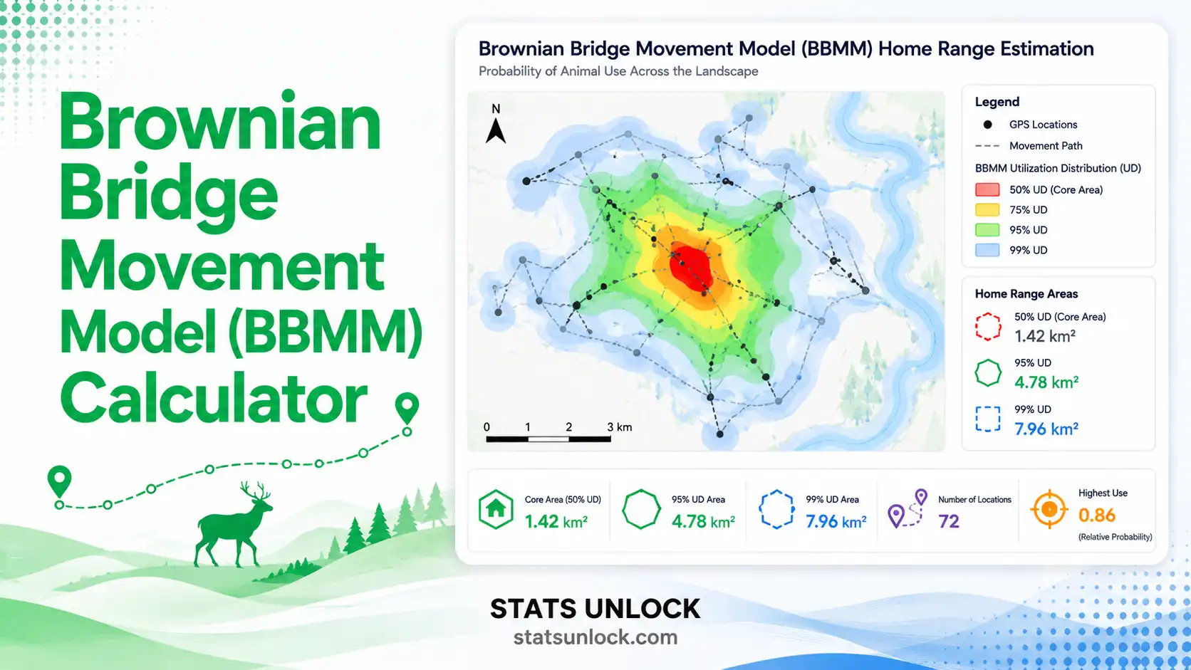
Brownian Bridge Movement Model Calculator (BBMM) – Free Online Home Range Estimator

📍 Data Input

Sample Dataset (USA wildlife examples)

Latitude values (decimal degrees, comma-separated)

0 values

Longitude values (decimal degrees, comma-separated)

0 values

Time intervals between consecutive fixes (minutes or hh:mm, comma-separated)

0 intervals — must equal (number of fixes − 1). Accepts decimal minutes (52, 61.5) or hh:mm format (1:30 = 90 min).

Upload CSV or Excel file (.csv, .txt, .xlsx, .xls)

Supports .csv, .txt, .xlsx, .xls — headers detected automatically. Map any three columns to Latitude, Longitude, and Δt (minutes) in one step.

Fix # Latitude Longitude Δt (min or hh:mm)

Δt is the time gap to the NEXT fix; the last row's Δt is unused. Accepts 60 or 1:00.

⚙️ Analysis Configuration

Study Group / Site / Individual Name (editable)

Used throughout interpretation, reports, and the research poster.

GPS Location Error σ²ₒ (m²)

Typical: 15–30 m²

Output Units (Area)

Grid Resolution

UD Contours

📊 Results

Brownian Bridge Movement Model Equation

The probability density at location z at time t, given start fix a at time t_a and end fix b at time t_b:

h(z | a, b, σ²m, σ²ₒ) ~ Normal( μ(t), σ²(t) )

μ(t) = a + α(b − a), α = (t − t_a) / (t_b − t_a)

σ²(t) = T · α(1 − α) · σ²m + (1 − α)² · σ²ₒ,a + α² · σ²ₒ,b

h: Brownian bridge probability density (utilization distribution kernel)
z: A candidate location on the grid where the animal could have been
a, b: Successive GPS fix locations (start and end of one segment)
t_a, t_b: Times of the two consecutive GPS fixes
T = (t_b − t_a): Time gap between consecutive fixes
α: Time fraction along the segment, where 0 = at start fix, 1 = at end fix
μ(t): Expected location at time t — straight-line interpolation
σ²(t): Movement variance at time t — widest at the midpoint of the segment
σ²m: Brownian motion variance — estimated by maximum likelihood from the GPS track
σ²ₒ: GPS location error variance (set in the configuration panel)
UD: Utilization distribution — sum of all bridge densities, normalised to integrate to 1

📋 Detailed Results Table

📈 Visualizations

1. UD Heatmap — Utilization Distribution

Density of animal occupancy across the grid (warmer colors = higher use)

2. GPS Track with 95%, 90%, 75% & 50% Contours

Movement track and nested utilization-distribution isopleths in space

3. Movement Speed Histogram

Distribution of step velocities (m/min) between consecutive fixes

4. Cumulative Area Curve (Sample-Size Asymptote)

Home range area growth as fixes accumulate — flattening = adequate sampling

📎 Copy summary statement to clipboard

🧭 Plain Language Interpretation

✍️ How to Write Your Results in Research

Five publication-style reporting templates with the latest BBMM values inserted automatically. Click 📋 Copy on any card to copy the text.

🪧 Research Poster Panel

A conference-ready visual layout. Drop into Canva, PowerPoint, or Illustrator and resize to A0 / A1 / 36×48 in.

📐 Technical Notes — Derivation, Assumptions & Limitations

1. How σ²m is Estimated

The Brownian motion variance σ²m is estimated by leave-one-out maximum likelihood (Horne et al., 2007). For each interior GPS fix z_i, predict its expected position as the linear interpolation between fixes z_i−1 and z_i+1; the residual variance summed over all interior fixes — corrected for the per-fix expected variance — gives the MLE of σ²m.

2. UD Construction

For every consecutive fix pair, the Brownian bridge density is evaluated at many interior time points (10–50 sub-intervals depending on segment length). Each evaluation contributes a 2-D Gaussian kernel to the UD grid. After summing all kernels across all segments, the grid is normalised so the total volume = 1.

3. Contour Extraction

UD cells are sorted by density in decreasing order; the smallest set of cells whose cumulative density equals 50% (core area) or 95% (home range) defines that isopleth. Area is computed by multiplying the number of cells by the cell area and converting to the chosen units.

4. Assumptions

Movement between consecutive fixes can be approximated by 2-D Brownian motion (random walk with normal step variance).
σ²m is constant across the entire track (relax this assumption by using dynamic BBMM / dBBMM).
GPS error is isotropic, normally distributed, and independent of true position.
Fix interval is short enough that consecutive locations are correlated (otherwise BBMM ≈ standard KDE).
The animal does not jump unrealistically between fixes; long gaps inflate σ² and may bias the UD.

5. Limitations

BBMM cannot recover habitat selection — it only describes where the animal was, not why.
Irregular fix schedules can bias σ²m; missing fixes should be flagged before analysis.
BBMM areas tend to be smaller than fixed-KDE areas because BBMM uses dynamic, time-aware bandwidths.
For migratory or behaviourally distinct tracks, segment the data or use dBBMM.
Edge effects: contours near the grid boundary should be checked; expand the grid extent if contours are truncated.

🎯 When to Use This Tool

Decision Checklist

✓ You have GPS telemetry data with timestamps for an individual animal
✓ Fix interval is regular (e.g., every 1 hr, 4 hr, 12 hr) and short relative to movement rate
✓ You have at least 30 fixes (100+ recommended for a stable estimate)
✓ You know or can estimate the GPS location error of your collar
✓ You want a time-aware home range, not just spatial point density
✗ Do NOT use if fixes are very sparse or irregular (use MCP or fixed KDE)
✗ Do NOT use if the animal underwent a clear behavioural shift mid-track (segment first, or use dBBMM)
✗ Do NOT use if you have presence-only or VHF triangulation data without precise timestamps

Real-World Examples (USA)

Gray Wolf Pack Dynamics (Yellowstone, WY) — Compare BBMM core areas between rendezvous-site phase and free-ranging phase to quantify den fidelity.
Florida Panther Corridor Planning — Use 95% BBMM home ranges across multiple panthers to identify pinch points between Big Cypress and protected satellite habitats.
Mule Deer Migration (Wyoming / Colorado) — Apply BBMM to a single GPS track to map seasonal migration corridors that standard KDE misses.
Brown Bear Foraging (Katmai NP, AK) — Compute monthly BBMM 50% core areas to identify salmon-stream concentration zones.

Sampling Design Guidance

Minimum 30 fixes per animal; 100+ for publication-grade estimates.
Fix interval ≤ 25% of the animal's average step time (consecutive fixes must be temporally correlated).
Avoid fix gaps > 4× the median interval — flag and consider splitting the track.
Record GPS error from collar manufacturer specifications (most modern collars: 15–25 m).
For seasonal comparisons, run BBMM separately on each biological season.

Related Methods Decision Tree

Just point density, ignore time? → Fixed kernel density estimation (KDE)
Simple area bound? → Minimum convex polygon (MCP 95%)
Movement varies over time? → Dynamic BBMM (dBBMM)
Need habitat selection too? → Step-Selection Functions (SSF) or Resource-Selection Functions (RSF)
Multiple animals, population-level UD? → AKDE (autocorrelated KDE)

🧰 How to Use This Tool — Step by Step

Enter your Study Group / Site / Individual Name (e.g., "Yellowstone Lamar Pack Wolf 921F").
Choose a sample dataset or upload your own GPS track (.csv / .xlsx). Use Column Entry mode if you prefer a labelled grid.
Paste latitudes and longitudes in decimal degrees, comma-separated. They must be the same length.
Enter Δt — the time gap (in minutes) between consecutive fixes. There should be one fewer Δt value than the number of fixes.
Set GPS location error σ²ₒ (default 20 m²; check your collar's specs).
Pick output area units (km² / ha / acres / mi²) and a grid resolution.
Choose which UD contours to compute (50% / 75% / 90% / 95%).
Click ▶ Calculate BBMM Home Range.
Inspect the four visualization plots — UD heatmap, GPS track with contours, speed histogram, and cumulative area curve.
Use the How to Write Your Results cards and the Research Poster panel to draft your report. Export with Download Doc or Download PDF.

Worked example (USA Gray Wolf, Yellowstone): 100 GPS fixes at hourly intervals over a Lamar Valley patrol yielded σ²m ≈ 1,800 m²/min, a 95% BBMM home range of ~ 380 km², and a 50% core of ~ 95 km², matching published estimates for the pack's summer range.

❓ Frequently Asked Questions

What is the Brownian Bridge Movement Model (BBMM)?

BBMM is a probabilistic home range estimator that uses GPS telemetry locations together with the time between fixes to estimate the distribution of likely locations between known points. The output is a utilization distribution (UD) — a 2-D probability surface representing how the animal used space over the tracking period.

How does BBMM differ from kernel density estimation (KDE)?

Standard KDE treats GPS points as independent samples and ignores time order. BBMM uses the timestamps and a Brownian motion variance parameter (σ²m) to weight where the animal likely was between fixes. This makes BBMM more accurate for animals with serially correlated movement and adaptive — animals with rapid movement get wider corridors, slow animals get narrower ones.

What is σ²m and how is it estimated?

σ²m is the Brownian motion variance — how much an animal wanders relative to a straight-line path between fixes. It is estimated by leave-one-out maximum likelihood from the GPS track itself: at each interior fix, the model predicts where the animal should be based on a straight line between its two neighbouring fixes; the variance of the residuals (corrected for fix interval) is the MLE of σ²m.

What is σ²ₒ (location error)?

σ²ₒ is the GPS error variance — typically 15–30 m² for modern collars. Set it according to your collar manufacturer's specifications. This tool defaults to 20 m², a reasonable assumption for typical Lotek / Vectronic / Telonics GPS collars.

What does the 95% home range mean?

The 95% utilization distribution contour encloses the smallest area within which the animal spent 95% of its tracked time. By convention, this is reported as the home range. The 50% contour is reported as the core area — the most intensively used region.

How many GPS fixes do I need for BBMM?

At least 30 fixes are needed for any meaningful estimate; 100 or more is the standard for publication-grade BBMM. The fix interval should be short enough that consecutive locations are correlated (otherwise BBMM degrades to a noisier version of KDE).

Can I use BBMM with VHF telemetry data?

BBMM is designed for high-frequency GPS data with regular fix intervals. VHF triangulations are usually too sparse and irregular, and they lack accurate timestamps. For VHF data, use minimum convex polygon (MCP) or fixed kernel density estimation instead.

What is dynamic BBMM (dBBMM) and when should I use it?

Standard BBMM assumes one σ²m for the whole track. Dynamic BBMM (dBBMM; Kranstauber et al., 2012) estimates a separate σ²m for each segment using a sliding window, capturing behavioural changes such as denning, migration, or foraging bouts. Use dBBMM when the track clearly shows distinct movement modes.

How do I report BBMM results in a journal paper?

Report (a) the 95% UD and 50% core area in km² or ha, (b) the estimated σ²m, (c) the number of GPS fixes and tracking duration, (d) the median fix interval, (e) the assumed location error σ²ₒ, and (f) cite Horne et al. (2007) for the BBMM method. Provide raw data on Movebank or an institutional repository for reproducibility.

Is BBMM appropriate for migratory or long-distance movement?

Yes — BBMM excels at migratory tracks because it explicitly models movement corridors that point-based methods like KDE miss. For seasonal comparisons run BBMM separately on each biological season. For tracks with clear behavioural switches (e.g., stopover, migration, post-arrival), use dBBMM.

🔍 Conclusion

▶ Run the analysis above to generate a personalised conclusion for your GPS telemetry dataset.

📚 References

Selected citations for the Brownian Bridge Movement Model, GPS telemetry home range estimation, and animal movement ecology, formatted in APA 7th edition.

Horne, J. S., Garton, E. O., Krone, S. M., & Lewis, J. S. (2007). Analyzing animal movements using Brownian bridges. Ecology, 88(9), 2354–2363. https://doi.org/10.1890/06-0957.1
Kranstauber, B., Kays, R., LaPoint, S. D., Wikelski, M., & Safi, K. (2012). A dynamic Brownian bridge movement model to estimate utilization distributions for heterogeneous animal movement. Journal of Animal Ecology, 81(4), 738–746. https://doi.org/10.1111/j.1365-2656.2012.01955.x
Bullard, F. (1991). Estimating the home range of an animal: A Brownian bridge approach [Master's thesis]. University of North Carolina at Chapel Hill.
Worton, B. J. (1989). Kernel methods for estimating the utilization distribution in home-range studies. Ecology, 70(1), 164–168. https://doi.org/10.2307/1938423
Calenge, C. (2006). The package "adehabitat" for the R software: A tool for the analysis of space and habitat use by animals. Ecological Modelling, 197(3–4), 516–519. https://doi.org/10.1016/j.ecolmodel.2006.03.017
Fleming, C. H., Fagan, W. F., Mueller, T., Olson, K. A., Leimgruber, P., & Calabrese, J. M. (2015). Rigorous home range estimation with movement data: A new autocorrelated kernel density estimator. Ecology, 96(5), 1182–1188. https://doi.org/10.1890/14-2010.1
Walter, W. D., Onorato, D. P., & Fischer, J. W. (2015). Is there a single best estimator? Selection of home range estimators using area-under-the-curve. Movement Ecology, 3(1), 10. https://doi.org/10.1186/s40462-015-0039-4
Sawyer, H., Kauffman, M. J., Nielson, R. M., & Horne, J. S. (2009). Identifying and prioritizing ungulate migration routes for landscape-level conservation. Ecological Applications, 19(8), 2016–2025. https://doi.org/10.1890/08-2034.1
Powell, R. A., & Mitchell, M. S. (2012). What is a home range? Journal of Mammalogy, 93(4), 948–958. https://doi.org/10.1644/11-MAMM-S-177.1
Cagnacci, F., Boitani, L., Powell, R. A., & Boyce, M. S. (2010). Animal ecology meets GPS-based radiotelemetry: A perfect storm of opportunities and challenges. Philosophical Transactions of the Royal Society B, 365(1550), 2157–2162. https://doi.org/10.1098/rstb.2010.0107
Nathan, R., Getz, W. M., Revilla, E., Holyoak, M., Kadmon, R., Saltz, D., & Smouse, P. E. (2008). A movement ecology paradigm for unifying organismal movement research. PNAS, 105(49), 19052–19059. https://doi.org/10.1073/pnas.0800375105
Silverman, B. W. (1986). Density Estimation for Statistics and Data Analysis. Chapman & Hall/CRC.
Seaman, D. E., & Powell, R. A. (1996). An evaluation of the accuracy of kernel density estimators for home range analysis. Ecology, 77(7), 2075–2085. https://doi.org/10.2307/2265701
Burt, W. H. (1943). Territoriality and home range concepts as applied to mammals. Journal of Mammalogy, 24(3), 346–352. https://doi.org/10.2307/1374834
Movebank Data Repository. https://www.movebank.org/ — Open repository of animal movement data including BBMM-ready GPS tracks.