KDE Home Range Estimator – Free Wildlife Calculator USA

📍 1. Data Input

Enter latitude / longitude coordinates of animal location fixes (GPS collar, VHF triangulation, or visual relocations). Decimal degrees, WGS84.

Study Area / Site Name (optional)

Species / Individual ID (Group Name)

📦 Use Sample Dataset

Latitude (decimal degrees, comma-separated) Longitude (decimal degrees, comma-separated)

0 location fixes parsed

Upload CSV or Excel file (.csv, .txt, .xlsx, .xls)

File must contain numeric latitude and longitude columns. Headers detected automatically.

Spreadsheet-style entry. Add/remove rows as needed.

#	Latitude	Longitude	Action

⚙️ 2. KDE Configuration

Tune the kernel and contour percentages before running the home range estimation.

Bandwidth Selector (h)

Manual Bandwidth (m) if Manual

Grid Resolution (cells per side)

Isopleth Contours Reported

95% Home Range 90% 75% 50% Core Area

All four isopleths are computed and reported by default.

Area Units

📊 3. Results — Home Range Summary

—

KDE Utilization Distribution Equation

The bivariate kernel density estimate at location x is:

\[ \hat{f}(\mathbf{x}) = \frac{1}{n\,h^2}\sum_{i=1}^{n} K\!\left(\frac{\mathbf{x} - \mathbf{x}_i}{h}\right) \]

f̂(x): estimated utilization distribution (probability density) at location x
n: number of independent animal location fixes
h: smoothing bandwidth (smoothing parameter) in meters
K(·): bivariate kernel function (Gaussian/normal kernel used here)
xᵢ: the i-th observed location (projected into a planar coordinate system in meters)
95% / 50% isopleth: contour enclosing the smallest area containing 95% / 50% of the volume of f̂

Statistic	Value	Description

📈 Visualizations

🗺️ 1. KDE Home Range Map — 95 / 90 / 75 / 50% Contours

📈 2. Cumulative Utilization Distribution Curve

📊 3. Isopleth Area Comparison — 50 / 75 / 90 / 95%

📍 4. Fix Distribution Histogram (Latitude & Longitude)

📎 Copy Summary to Clipboard

🧭 4. Plain Language Interpretation

Detailed ecological reading of the result — auto-fills with your data.

✍️ How to Write Your Results in Research (5 Templates + Poster)

📘 Ecology Journal Style

Key conventions

Use italicised symbols (h, UD). Always state n (fixes), the bandwidth method, the kernel, and the isopleth %. Cite Worton (1989) and Seaman & Powell (1996).

🎓 Thesis / Dissertation Style

Key conventions

Include a Methods mini-paragraph naming the software (e.g., adehabitatHR in R; kernelUD function). State sampling effort, fix interval, and independence test. Report both 95% and 50% isopleths.

📑 Plain-Language / Policy Brief

Key conventions

Avoid all symbols. Translate the result into "the animal regularly used X hectares of land." Include a management implication as the final sentence.

🪧 Conference Abstract

Key conventions

Four labelled sections: Background, Methods, Results, Conclusion. Strict 150–250 word limit. Always state n and bandwidth.

🔭 LTER / Monitoring Report

Key conventions

Compare against the previous reporting period or baseline. Always include sampling effort (fix interval × days). Note any change in home range size and possible drivers.

🪧 Research Poster Panel

Home Range of [Species] at [Site Name]

🌍 Introduction

🧪 Methods

📊 Key Results

— ha

95% KDE Home Range

90% Isopleth

—

75% Isopleth

—

50% Core Area

—

Fixes (n)

—

Bandwidth h

—

Core:HR Ratio

—

💬 Discussion

🎯 Conclusions

📚 Footer / References / Contact

🎨 Poster Design Specifications

Typography: Title 72–96 pt (Montserrat/DM Sans Bold); section headers 36–48 pt; body 24–28 pt (24 pt absolute minimum at 1 m viewing distance); callout numbers 60–80 pt.

Colour palette: White background; deep forest green (#1f6e47) for headers and callout borders; amber (#d97706) for comparisons; muted red (#dc2626) for cautionary notes. Maximum 3 accent colours.

Sizes: A0 portrait 841×1189 mm, A0 landscape 1189×841 mm, 36×48 in (North American standard), A1 portrait 594×841 mm.

Resolution: 300 dpi minimum; export as PDF/X-1a (not PNG) for professional print.

Software: Canva (free), PowerPoint, Adobe Illustrator, Inkscape.

🔍 5. Detailed Conclusion

▶ Run the analysis above to generate a personalised conclusion for your dataset.

📐 Technical Notes — Bandwidth, Kernels, and Assumptions

Reference (h_ref) bandwidth: For a bivariate normal kernel, h_ref = σ · n^−1/6, where σ is the pooled standard deviation of the two coordinate axes. This estimator is appropriate when the underlying utilization distribution is approximately bivariate normal and is the most commonly reported method in wildlife studies (Worton, 1989).

Least Squares Cross-Validation (h_LSCV): Selects bandwidth by minimising the mean integrated squared error. Can fail to converge for highly autocorrelated data — common in modern GPS collars with short fix intervals.

Plug-in bandwidth (h_pi): Two-stage estimator (Sheather & Jones, 1991) that is generally less biased than h_ref when the UD is multimodal.

Assumptions: independent fixes, no positional error, animal home range is closed (no migration), kernel is appropriate for the spatial scale of movement.

Limitations: KDE assumes spatial independence of fixes which is rarely met by GPS data sampled every < 4 h. Autocorrelated data inflates the perceived home range. Consider Autocorrelated KDE (AKDE; Fleming et al., 2015) for high-frequency telemetry.

✅ When to Use This KDE Home Range Estimator

Decision checklist

✓ You have ≥ 30 independent location fixes from one animal
✓ You want a probabilistic (not just polygon) home range estimate
✓ You need both home range (95%) and core area (50%) reported
✓ You want a publication-ready KDE home range result for a US wildlife journal
✗ Do NOT use if < 20 fixes are available — use MCP instead
✗ Do NOT use raw KDE for high-frequency GPS data without checking autocorrelation — use AKDE
✗ Do NOT use for migratory animals across full annual cycle — partition by season first

Real-world examples (USA)

Mule deer in Colorado: seasonal home range partitioning across winter and summer ranges
Florida black bear: male vs. female home range size comparison for connectivity planning
Mountain lion in California: core area overlap with urban-wildland interface
Wild turkey in Texas: brood-rearing home range during nesting season

Sampling design guidance

Minimum 30 fixes per animal; 50–100+ preferable for stable KDE
Fix interval should be long enough for biological independence (typically ≥ 4 h)
Sample across the full activity cycle (day + night)
Pool fixes by individual, season, or sex before estimating

Related home range estimators

Need a deterministic polygon? → MCP (Minimum Convex Polygon)
High-frequency GPS with autocorrelation? → AKDE (Autocorrelated KDE)
Movement-based weighting? → Brownian Bridge MM (BBMM)
Local convex hulls? → LoCoH (k-NN, a-LoCoH, r-LoCoH)

📘 How to Use This Tool — Step-by-Step

Enter your data: paste latitude/longitude as comma-separated values, upload a CSV/Excel file, or use the manual table. The textarea expects values like: 40.4523, 40.4531, 40.4519, ...
Choose a sample dataset: 5 ecological datasets (mule deer, coyote, black bear, mountain lion, wild turkey) are available from the dropdown.
Configure bandwidth: use Reference (h_ref) by default. Select LSCV or plug-in for advanced cases.
Set isopleths: the standard convention is 95% home range and 50% core area.
Click "Run KDE Home Range Analysis": nothing runs on page load — you must click the button.
Read summary cards: green = full home range; amber = core area; deep green = bandwidth.
Read the full results table: includes all metric components, n, bandwidth, isopleth areas.
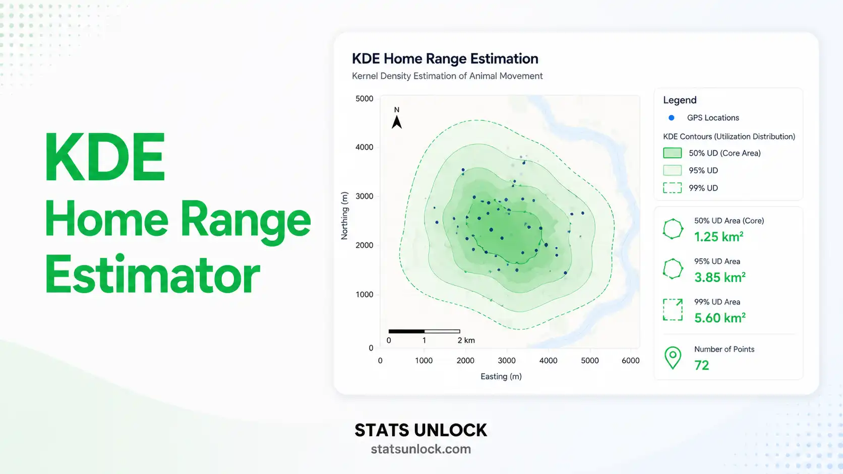
Examine the four visualisations: KDE map, UD curve, isopleth-area curve, fix histogram.
Copy the right reporting template: journal, dissertation, plain language, abstract, monitoring, or full research poster.
Export your results: Doc (.txt) for editing or PDF for printing/sharing.

Worked example: A wildlife biologist tracks one female mule deer in Routt County, Colorado, with a GPS collar transmitting every 4 hours for 30 days, yielding 180 location fixes. Pasting the lat/lon columns, running KDE with h_ref and the 95%/50% defaults, returns a 95% home range of approximately 240 ha and a 50% core area of approximately 45 ha — typical for adult mule deer in mountain shrubland habitat.

❓ Frequently Asked Questions about KDE Home Range Estimation

What is kernel density estimation (KDE) in wildlife ecology?

KDE is a non-parametric statistical method that estimates a smooth probability density function (the utilization distribution) from a set of discrete animal location points. The 95% isopleth of this density defines the home range, and the 50% isopleth defines the core area (Worton, 1989).

What is the difference between the 95% and 50% home range?

The 95% isopleth encloses the area within which the animal is found 95% of the time — the conventional home range definition. The 50% isopleth represents the most intensively used half of the utilization distribution — the core area, often interpreted as primary habitat or refuge.

How many GPS fixes do I need for a reliable KDE?

A minimum of 30 independent location fixes is recommended; 50–100+ produces more stable estimates. With fewer than 20 fixes, KDE results are unreliable and the Minimum Convex Polygon (MCP) is a safer choice.

Which bandwidth selector should I use?

Reference bandwidth (h_ref) is the most reported method and is appropriate for unimodal home ranges. Least Squares Cross-Validation (LSCV) can reduce oversmoothing but often fails with autocorrelated data. Plug-in bandwidth performs well with multi-modal UDs.

Can I use latitude and longitude directly with KDE?

Yes — this tool accepts decimal-degree lat/lon, then internally projects to a local equal-area frame in meters so the resulting areas are correct in hectares, km², or acres. For studies spanning > 100 km, a formal projection (e.g., UTM, Albers Equal Area) is recommended.

What does it mean when LSCV fails to converge?

It usually means the GPS fixes are spatially autocorrelated (too close in time). In that case the algorithm is unable to find a finite minimum and either fails or returns an unrealistically small bandwidth. Switch to h_ref or use AKDE.

What is autocorrelated KDE (AKDE) and when do I need it?

AKDE (Fleming et al., 2015) accounts for the temporal autocorrelation of modern GPS data. It is the gold standard for fix intervals shorter than the animal's typical mean revisit time (i.e., most GPS collars at 1–4 h fix rates).

Is KDE better than Minimum Convex Polygon (MCP)?

KDE is probabilistic and reports both the home range and core area, while MCP is a deterministic outer hull. KDE is preferred for ecological inference, but MCP remains the international comparability standard required by many older studies and management plans.

How do I report a KDE home range in a manuscript?

Always report n (fixes), bandwidth method, kernel type, isopleth %, area + units, and the software used. Example: "95% KDE home range = 240 ha (h_ref = 95 m, Gaussian kernel, n = 180 fixes, calculated in adehabitatHR R package; Calenge, 2006)."

Is this KDE home range tool free for US wildlife researchers?

Yes — this tool is 100% free, runs entirely in the browser, requires no signup, and is optimised for US wildlife biologists working on deer, bear, coyote, mountain lion, wild turkey, and similar species.

📚 References

Foundational and methodological sources for kernel density estimation, bandwidth selection, autocorrelated KDE, and comparison with alternative home range estimators.

Worton, B. J. (1989). Kernel methods for estimating the utilization distribution in home-range studies. Ecology, 70(1), 164–168. https://doi.org/10.2307/1938423
Seaman, D. E., & Powell, R. A. (1996). An evaluation of the accuracy of kernel density estimators for home range analysis. Ecology, 77(7), 2075–2085. https://doi.org/10.2307/2265701
Seaman, D. E., Millspaugh, J. J., Kernohan, B. J., Brundige, G. C., Raedeke, K. J., & Gitzen, R. A. (1999). Effects of sample size on kernel home range estimates. Journal of Wildlife Management, 63(2), 739–747. https://doi.org/10.2307/3802664
Silverman, B. W. (1986). Density Estimation for Statistics and Data Analysis. Chapman & Hall.
Calenge, C. (2006). The package adehabitat for the R software: a tool for the analysis of space and habitat use by animals. Ecological Modelling, 197, 516–519. https://doi.org/10.1016/j.ecolmodel.2006.03.017
Fleming, C. H., Fagan, W. F., Mueller, T., Olson, K. A., Leimgruber, P., & Calabrese, J. M. (2015). Rigorous home range estimation with movement data: a new autocorrelated kernel density estimator. Ecology, 96(5), 1182–1188. https://doi.org/10.1890/14-2010.1
Kie, J. G., Matthiopoulos, J., Fieberg, J., Powell, R. A., Cagnacci, F., Mitchell, M. S., Gaillard, J.-M., & Moorcroft, P. R. (2010). The home-range concept: are traditional estimators still relevant with modern telemetry technology? Philosophical Transactions of the Royal Society B, 365(1550), 2221–2231. https://doi.org/10.1098/rstb.2010.0093
Powell, R. A. (2000). Animal home ranges and territories and home range estimators. In L. Boitani & T. K. Fuller (Eds.), Research Techniques in Animal Ecology (pp. 65–110). Columbia University Press.
Sheather, S. J., & Jones, M. C. (1991). A reliable data-based bandwidth selection method for kernel density estimation. Journal of the Royal Statistical Society B, 53(3), 683–690. https://doi.org/10.1111/j.2517-6161.1991.tb01857.x
Gitzen, R. A., Millspaugh, J. J., & Kernohan, B. J. (2006). Bandwidth selection for fixed-kernel analysis of animal utilization distributions. Journal of Wildlife Management, 70(5), 1334–1344. https://doi.org/10.2193/0022-541X(2006)70[1334:BSFFAO]2.0.CO;2
Walter, W. D., Onorato, D. P., & Fischer, J. W. (2015). Is there a single best estimator? Selection of home range estimators using area-under-the-curve. Movement Ecology, 3, 10. https://doi.org/10.1186/s40462-015-0039-4
Laver, P. N., & Kelly, M. J. (2008). A critical review of home range studies. Journal of Wildlife Management, 72(1), 290–298. https://doi.org/10.2193/2005-589
R Core Team. (2024). R: A language and environment for statistical computing. R Foundation for Statistical Computing. https://www.R-project.org/
Signer, J., Fieberg, J., & Avgar, T. (2019). Animal movement tools (amt): R package for managing tracking data and conducting habitat selection analyses. Ecology and Evolution, 9(2), 880–890. https://doi.org/10.1002/ece3.4823
Burt, W. H. (1943). Territoriality and home range concepts as applied to mammals. Journal of Mammalogy, 24(3), 346–352. https://doi.org/10.2307/1374834