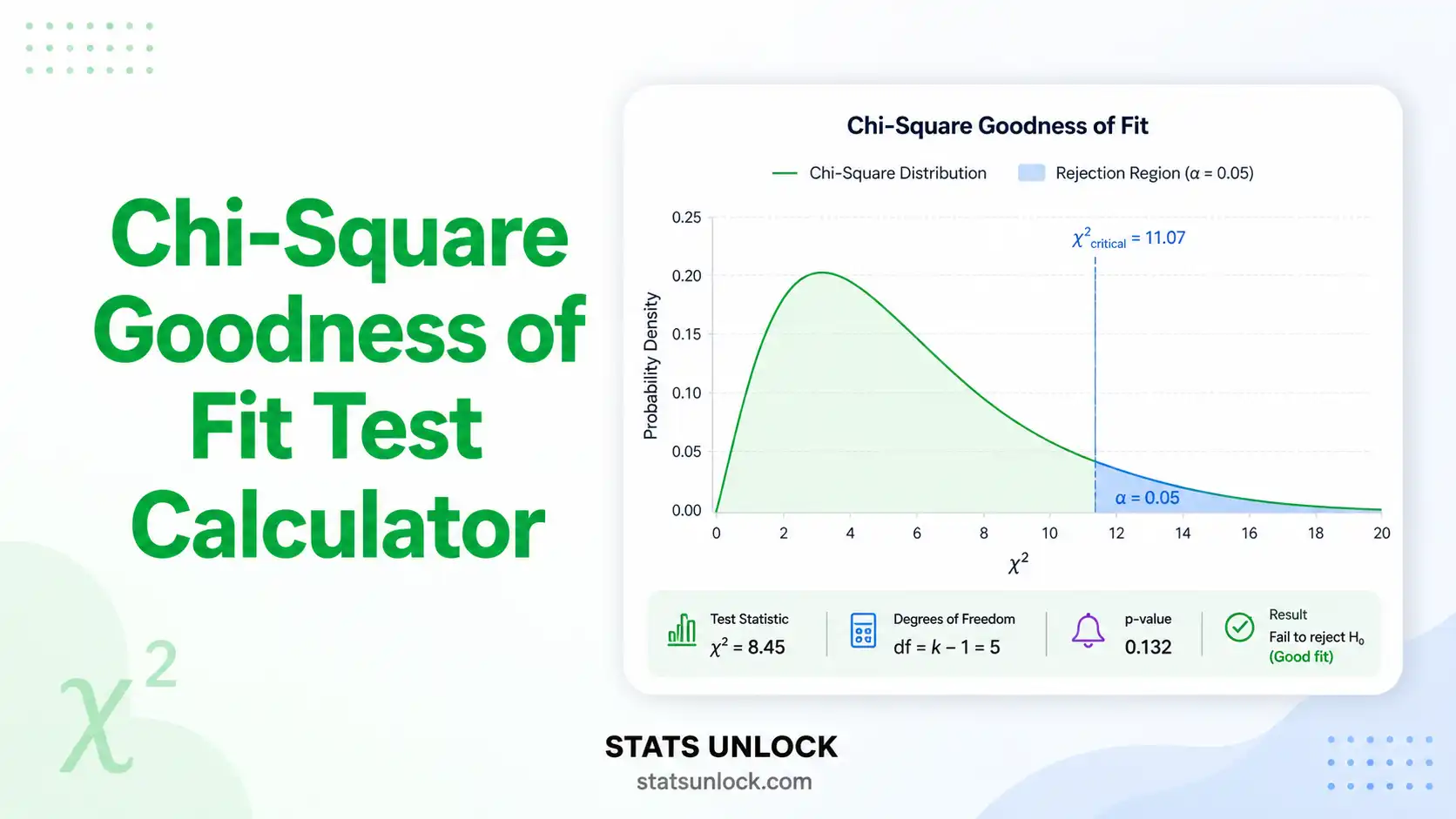
Chi-Square Goodness of Fit Test Calculator (Free) | StatsUnlock

Chi-Square Goodness of Fit Test Calculator (Free) | StatsUnlock
StatsUnlock · Hypothesis Tests

Chi-Square Goodness of Fit
Test Calculator

A free online chi-square goodness of fit test calculator. Enter observed frequencies, compare them to expected counts, and instantly get the chi-square statistic, p-value, Cramér's V effect size, standardized residuals, and an APA-format result string — all in one click.

non-parametric · single categorical variable · χ² distribution
FreeOnlinep-valueEffect sizeAPA formatColorful charts
📊 Enter Your Data
Each name labels one category. Edit freely — these display in tables and charts.
A label for the dataset, shown in results and exports.
One non-negative integer per category. Counts must be in the same order as the category names above.
Category Name Observed Count
⚙️ Test Configuration
Subtract 1 df per parameter you estimated from the data (e.g., mean, variance for fitting Normal/Poisson).
Results Summary

📋 Full Statistical Results

🔢 Observed vs Expected Frequencies

Standardized residuals greater than ±1.96 (highlighted) indicate categories that contribute most to the chi-square statistic.

🎨 Colorful Visualizations

Observed vs Expected Frequencies
Standardized Residuals by Category
Per-Category Contribution to χ²
χ² Distribution with Critical Region

🔎 Assumption Checks

    📖 Detailed Interpretation of Results
    ✍️ How to Write Your Results in Research
    🎯 Conclusion
    🧮 Formulas & Technical Notes

    Test Statistic — Pearson's Chi-Square

    χ² = Σ [ (Oᵢ − Eᵢ)² / Eᵢ ]
    Where: χ² = Pearson chi-square test statistic Oᵢ = observed frequency in category i Eᵢ = expected frequency in category i (under H₀) Σ = sum across all k categories

    Degrees of Freedom

    df = k − 1 − m
    Where: k = number of categories m = number of parameters estimated from the data (default 0 if expected counts come from theory)

    Standardized Residual (per cell)

    zᵢ = (Oᵢ − Eᵢ) / √Eᵢ
    Where: zᵢ = standardized residual for category i |zᵢ| > 1.96 indicates that category contributes meaningfully to a significant χ² at α = .05

    Effect Size — Cramér's V (one-variable case)

    V = √( χ² / (N · (k − 1)) )
    Where: V = Cramér's V (also reported as φ when k = 2) N = total sample size (sum of observed counts) k = number of categories Cohen's benchmarks for one-variable Cramér's V: 0.10 small, 0.30 medium, 0.50 large.

    Yates' Continuity Correction (only for df = 1)

    χ²_yates = Σ [ (|Oᵢ − Eᵢ| − 0.5)² / Eᵢ ]
    Where: applied only when df = 1 to reduce upward bias of the discrete chi-square approximation. Not used for df ≥ 2.

    Technical Notes

    • The test statistic follows a χ² distribution with df = k − 1 − m under the null hypothesis.
    • The p-value is computed from the upper tail: P(χ² > observed | df).
    • If any expected count Eᵢ < 5 in more than 20% of cells, the χ² approximation may be unreliable; consider Fisher's exact test or Monte Carlo simulation.
    • Yates' correction is applied only for df = 1 and is conservative — it reduces Type I error but lowers power.
    📌 When to Use This Test

    This free chi-square goodness of fit test calculator is designed for testing whether observed frequencies in a single categorical variable match a hypothesized distribution. It answers the question: does my sample come from the population I think it does?

    Decision Checklist

    • You have one categorical variable with two or more mutually exclusive categories
    • Your data are frequencies (counts), not means or proportions
    • Each observation belongs to exactly one category (mutually exclusive)
    • Observations are independent of each other
    • Expected count in each category is at least 5 (or 1 in ≤20% of cells)
    • Do NOT use if you have two categorical variables → use Chi-Square Test of Independence
    • Do NOT use if your data are continuous → use Kolmogorov-Smirnov or Anderson-Darling
    • Do NOT use if observations are paired/repeated on the same subjects → use McNemar's test
    • Do NOT use if expected counts are very small (<1 in any cell) → use Fisher's exact test

    Real-World Examples

    1. Genetics — Mendelian inheritance: A geneticist crosses two heterozygous pea plants and counts 315 round-yellow, 101 wrinkled-yellow, 108 round-green, 32 wrinkled-green offspring. Test whether these counts match the theoretical 9:3:3:1 ratio.
    2. Quality control — die fairness: A casino auditor rolls a die 600 times and records frequencies for faces 1–6. Test whether the die is fair (each face expected at 1/6 = 100 times).
    3. Marketing — consumer preference: A company tests five flavors of ice cream. From 500 surveyed customers, observe how many prefer each flavor. Test whether preferences are equally distributed (uniform null) or whether some flavors are preferred.
    4. Wildlife ecology — habitat selection: A camera-trap study records 240 detections of leopards across four habitat types (forest, grassland, scrub, agriculture). Test whether detections deviate from random use proportional to habitat availability.
    5. Education — multiple choice answer keys: A teacher analyzes 100-item answer keys to test whether correct answers (A, B, C, D) are uniformly distributed, as a check for test-construction bias.

    Sample Size Guidance

    Minimum recommended total N: at least 5 × k (so each category's expected count ≥ 5). For small effect detection (V ≈ 0.10), aim for N ≥ 200; for medium (V ≈ 0.30), N ≥ 90; for large (V ≈ 0.50), N ≥ 40.

    Decision Tree — Choosing the Right Test

    One categorical variable → THIS TEST (Chi-Square Goodness of Fit)
                             → Small expected counts (<5 in many cells) → Fisher's exact / Monte Carlo
    Two categorical variables → Chi-Square Test of Independence
                             → 2×2 small N → Fisher's exact test
                             → Paired binary outcomes → McNemar's test
    Continuous data → Normality? → Shapiro-Wilk / Anderson-Darling / Kolmogorov-Smirnov
            
    📘 How to Use This Chi-Square Goodness of Fit Calculator — Step-by-Step
    01

    Enter Your Data

    Choose one of three input methods: type/paste comma-separated counts (default), upload a CSV/Excel file and pick which column holds the category names and which holds the observed counts, or use the manual entry table. Every method results in the same data being analyzed.

    02

    Choose a Sample Dataset (Optional)

    Five built-in datasets cover the most common use cases: dice fairness, Mendelian 9:3:3:1 inheritance, customer preference, Likert survey distribution, and wildlife habitat selection. Sample 1 (Dice Rolls) loads by default.

    03

    Set Category Names and Group Name

    Edit the comma-separated category names — these label every table, axis, and chart. Edit the group name to label your dataset (e.g., "Dice rolls", "Pea plants", "Leopard detections") — it shows up in the results, exports, and APA write-up.

    04

    Choose Your Expected Frequency Model

    Three options: Uniform (equal counts across categories — the default for fairness tests), Custom proportions (e.g., 9:3:3:1 for Mendelian, will be normalized automatically), or Custom counts (enter expected frequencies directly).

    05

    Configure the Test

    Choose α (default 0.05). If you estimated parameters from your data (e.g., the mean for fitting a Poisson distribution), increase the df reduction. Yates' continuity correction is only for df = 1 cases.

    06

    Click "Run Chi-Square Goodness of Fit Test"

    Calculation is instant. Results, four colorful visualizations, residuals table, and assumption checks appear below.

    07

    Read the Summary Cards

    Four colour-coded cards show χ², df, p-value, and Cramér's V. Green = significant at α; amber = non-significant. The cards are the at-a-glance verdict.

    08

    Inspect the Visualizations

    Chart 1 (bars) compares observed vs expected counts. Chart 2 (residuals) shows which categories drive significance — bars beyond ±1.96 are flagged. Chart 3 (donut) shows each category's % contribution to χ². Chart 4 (curve) plots the χ² distribution with the critical region shaded.

    09

    Check Assumptions

    Three pass/warn/fail badges report (a) sample size adequacy, (b) expected count rule (≥ 5 per cell), and (c) independence. Always satisfy all three before reporting your result.

    10

    Export Your Results

    Click "Download Doc" for a plain-text .txt report (paste into Word or Google Docs). Click "Download PDF" to print a clean A4-formatted PDF. Use "Copy summary statement" to grab the APA-ready one-liner for your manuscript.

    ❓ Frequently Asked Questions
    Q1. What is the chi-square goodness of fit test and when should I use it?
    The chi-square goodness of fit test compares observed category frequencies in a single sample to expected frequencies derived from a theoretical distribution. Use it whenever you have one categorical variable and want to test whether the data match a known distribution — for example, testing whether dice rolls are uniform, whether a genetic cross fits Mendelian ratios, or whether survey responses follow a 5-point Likert distribution.
    Q2. What is the difference between chi-square goodness of fit and chi-square test of independence?
    Goodness of fit uses one categorical variable and compares observed counts to a hypothesized distribution. The test of independence uses two categorical variables in a contingency table and tests whether they are associated. The test statistic and distribution are similar, but the research question differs entirely.
    Q3. What are the assumptions of the chi-square goodness of fit test?
    Independent observations, mutually exclusive categories, frequency data (counts, not proportions or means), and an expected frequency of at least 5 in each cell. Some references allow up to 20% of cells to have expected counts between 1 and 5, but no cell should be below 1.
    Q4. How do I interpret a significant result?
    A significant p-value (p < α) means the observed frequencies differ significantly from the expected frequencies under the null hypothesis. Examine the standardized residuals to identify which categories drive the difference — values beyond ±1.96 indicate categories contributing most to the chi-square statistic at α = 0.05.
    Q5. What effect size should I report?
    Report Cramér's V (or φ for k = 2). For one-variable goodness of fit, Cohen's benchmarks are V = 0.10 small, V = 0.30 medium, V = 0.50 large. Effect size is mandatory in modern reporting because a large N can make trivial differences statistically significant.
    Q6. What are degrees of freedom for chi-square goodness of fit?
    df = k − 1 − m, where k is the number of categories and m is the number of parameters you estimated from the data. If your expected counts come purely from theory (no parameters estimated), m = 0 and df = k − 1. If you estimated, say, the Poisson mean from your data to compute expected counts, m = 1.
    Q7. Can I test for a uniform distribution?
    Yes. Select "Uniform" as the expected frequency model. This sets all expected counts equal to N/k. The test then evaluates whether observed counts deviate from equal distribution across categories.
    Q8. What if my expected frequencies are below 5?
    The chi-square approximation becomes unreliable. Solutions: (a) combine adjacent or sparse categories into broader groups, (b) collect more data, or (c) use Fisher's exact test or a Monte Carlo simulation, both of which give exact p-values without needing the asymptotic approximation.
    Q9. Is chi-square goodness of fit parametric or non-parametric?
    Non-parametric. It does not assume the response variable is normally distributed; it uses categorical frequency data and relies only on the asymptotic χ² distribution of the test statistic under H₀. This is why it is grouped with non-parametric tests in most curricula.
    Q10. How do I report the result in APA 7th edition format?
    Format: χ²(df, N = total) = test statistic, p = p-value, V = effect size. Example: "A chi-square goodness of fit test indicated that observed frequencies differed significantly from expected, χ²(5, N = 320) = 12.45, p = .029, V = .20." Always report N, df, exact p (or "p < .001"), and an effect size.
    📚 References

    The following references support the statistical methods used in this chi-square goodness of fit test calculator, covering p-value interpretation, effect size reporting, and best practices in hypothesis testing with categorical data.

    1. Pearson, K. (1900). On the criterion that a given system of deviations from the probable in the case of a correlated system of variables is such that it can be reasonably supposed to have arisen from random sampling. Philosophical Magazine, 50(302), 157–175. https://doi.org/10.1080/14786440009463897
    2. Yates, F. (1934). Contingency tables involving small numbers and the χ² test. Supplement to the Journal of the Royal Statistical Society, 1(2), 217–235. https://doi.org/10.2307/2983604
    3. Cochran, W. G. (1954). Some methods for strengthening the common χ² tests. Biometrics, 10(4), 417–451. https://doi.org/10.2307/3001616
    4. Cohen, J. (1988). Statistical power analysis for the behavioral sciences (2nd ed.). Lawrence Erlbaum Associates.
    5. Cramér, H. (1946). Mathematical methods of statistics. Princeton University Press.
    6. Agresti, A. (2018). An introduction to categorical data analysis (3rd ed.). John Wiley & Sons.
    7. Field, A. (2018). Discovering statistics using IBM SPSS statistics (5th ed.). SAGE Publications.
    8. Howell, D. C. (2013). Statistical methods for psychology (8th ed.). Cengage Learning.
    9. McHugh, M. L. (2013). The chi-square test of independence. Biochemia Medica, 23(2), 143–149. https://doi.org/10.11613/BM.2013.018
    10. Sharpe, D. (2015). Chi-square test is statistically significant: Now what? Practical Assessment, Research & Evaluation, 20(8), 1–10. https://doi.org/10.7275/tbfa-x148
    11. Lakens, D. (2013). Calculating and reporting effect sizes to facilitate cumulative science. Frontiers in Psychology, 4, 863. https://doi.org/10.3389/fpsyg.2013.00863
    12. American Psychological Association. (2020). Publication manual of the American Psychological Association (7th ed.). APA. https://doi.org/10.1037/0000165-000
    13. R Core Team. (2024). R: A language and environment for statistical computing. R Foundation for Statistical Computing. https://www.R-project.org/
    14. NIST/SEMATECH. (2013). e-Handbook of statistical methods — Chi-square goodness of fit test. https://www.itl.nist.gov/div898/handbook/eda/section3/eda35f.htm
    15. Virtanen, P., Gommers, R., Oliphant, T. E., et al. (2020). SciPy 1.0: Fundamental algorithms for scientific computing in Python. Nature Methods, 17, 261–272. https://doi.org/10.1038/s41592-020-0772-5

    Leave a Reply

    Your email address will not be published. Required fields are marked *

    Previous Post
    Next Post

    © 2026 STATS UNLOCK . statsunlock.com –  All Rights Reserved.