

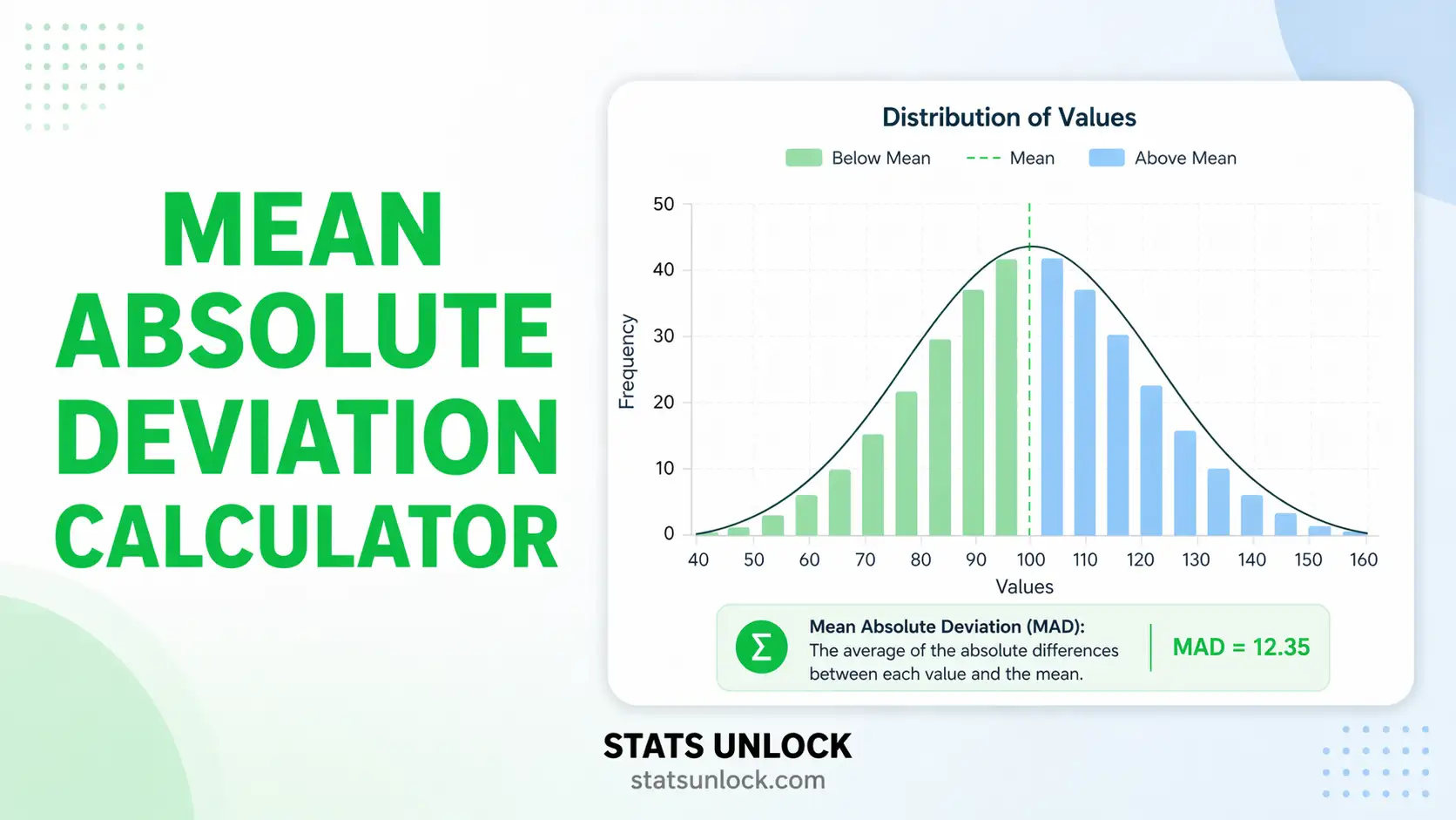

Paste comma-separated numbers and get the mean absolute deviation (MAD), median absolute deviation, standard deviation, coefficient of variation, four colourful charts and ready-to-paste APA sentences, free, instant, no sign-up.
⚡ 0. Quick Answer
Mean absolute deviation tells you how far a typical value sits from the mean, on average, ignoring whether it is above or below. Add up the absolute gaps between each value and the mean, then divide by how many values you have. The answer is in the same units as your data, dollars stay dollars, kilograms stay kilograms.
Rule of thumb: MAD = 0 means every value is identical. For roughly normal data MAD ≈ 0.798 × SD, so a MAD/SD ratio near 0.80 suggests normal-shaped data, while a ratio below 0.70 flags heavy tails or outliers.
🔑 Key Takeaways
- This mean absolute deviation calculator returns MAD, median absolute deviation, SD, variance, range, IQR and CV from one comma-separated paste.
- MAD divides by n, never n−1, Bessel's correction belongs to variance and standard deviation only.
- For normal data MAD ≈ 0.798 × SD; a ratio far below that means outliers are inflating the SD.
- The most common mistake is dropping the absolute-value bars, the raw deviations always sum to exactly 0.
- Report MAD in the same units as the data, alongside the mean, and use CV only when all values are positive.
- Median absolute deviation (about the median) is the robust twin, use it when a single extreme value dominates.
📘 1. What Is Mean Absolute Deviation?
The mean absolute deviation (MAD, also called average absolute deviation or mean deviation) is a measure of spread. It answers a simple question: on average, how far is a value from the centre of the data? Because it uses absolute values, distances above and below the mean count equally and never cancel out. The result is easy to explain to a non-statistician: "on average, readings sit 4.2 units away from the mean."
What it measures
- MAD, average distance from the mean, in the original data units.
- Median absolute deviation, median distance from the median, in the same units; robust to outliers.
- Relative MAD (CV of MAD), MAD divided by the mean, expressed as a percentage; unit-free.
- MAD/SD ratio, a quick shape diagnostic; near 0.798 for a normal distribution.
- Total absolute deviation, the numerator Σ|xᵢ − x̄|, useful for hand-checking.
A worked one-liner
If five readings are 52, 48, 55, 61, 47 the mean is 52.6. The absolute gaps are 0.6, 4.6, 2.4, 8.4, 5.6, which sum to 21.6. Divide by 5 and MAD = 4.32, a typical reading sits about 4.3 units from the mean.
Who uses it
Middle-school and high-school curricula (Common Core 6.SP.B.5c) introduce spread with MAD before standard deviation because it needs no squaring. Forecasters use the closely related Mean Absolute Error to score predictions. Quality engineers, ecologists reporting count variability, and finance analysts describing dispersion in returns all use MAD when they want a figure that is easy to explain in plain units.
How it differs from the nearest alternatives
| Measure | How it treats distance | Pick it when |
|---|---|---|
| Mean absolute deviation | Averages the absolute gaps from the mean | You want a plain-units, easy-to-explain spread that is not dominated by one extreme value |
| Standard deviation | Averages squared gaps, then square-roots | You need the input to a t-test, ANOVA, CI or any normal-theory method |
| Median absolute deviation | Median of absolute gaps from the median | Outliers are present and you want the most robust spread available |
🧮 2. Set Up Your Data
📊 3. Results
🔍 4. Interpretation of Results, In Detail
4.6 Decision guide: what to do with your MAD
| What you see | What it means | What to do next |
|---|---|---|
| MAD = 0 | Every value is identical; there is no variability at all | Check for a copy-paste error or a constant column before reporting |
| MAD very small relative to the mean (CV < 5%) | The mean summarises the data very well | Report the mean with confidence; the MAD is a supporting detail |
| MAD large relative to the mean (CV > 40%) | The mean is a weak summary; individual values differ a lot | Report the median and IQR alongside, and inspect the histogram for subgroups |
| MAD/SD ratio ≈ 0.75–0.85 | Consistent with a roughly normal shape | Normal-theory methods (t-test, CI on the mean) are reasonable |
| MAD/SD ratio < 0.70 | Heavy tails or at least one strong outlier is inflating SD | Report the median absolute deviation as the primary spread; consider robust methods |
| MAD/SD ratio > 0.90 | Very light tails, often uniform, bimodal or bounded data | Plot the histogram; a normal model may be a poor fit |
| MAD ≫ median absolute deviation | A small number of extreme values dominate the mean-based figure | Identify the outliers, decide (and pre-register) whether they are genuine |
| Two groups, similar means but very different MADs | Equal averages, unequal consistency | Report both; a difference in spread can matter more than a difference in means |
4.7 Common mistakes this calculator prevents
- Forgetting the absolute-value bars. Signed deviations from the mean always sum to exactly zero, so the "average deviation" without absolute values is always 0. The calculator shows the signed sum so you can verify this.
- Dividing by n − 1. Bessel's correction exists to make the variance unbiased. It has no justification for MAD. This tool always divides by n and states so on screen.
- Confusing the two MADs. "MAD" means mean absolute deviation here; in robust statistics it often means median absolute deviation. Both are computed and labelled separately so you never quote the wrong one.
- Comparing MADs across different units. A MAD of 4 kg and a MAD of 4 grams are not comparable. Use the relative MAD (percentage of the mean) for cross-scale comparison, which is shown in the results table.
- Reporting MAD to more decimals than the raw data. If your readings have one decimal place, MAD to six decimals is false precision. The decimal-places selector lets you match your instrument.
- Treating MAD as an inference statistic. MAD describes the sample you have. It is not a test, has no p-value, and by itself says nothing about a population.
✍️ 5. How to Write Your Results in Research
When reporting mean absolute deviation calculator output in a paper, thesis or report, always pair the MAD with the mean and the sample size, state the units, and say explicitly which centre you used. Five ready-to-paste templates follow; press Copy on the one that matches your outlet.
5.6 Table and figure conventions
- In a descriptive table, give one row per group with columns: n, M, SD, MAD, Mdn, IQR. Align decimals and use the same precision throughout.
- Define MAD in the table note the first time it appears: "MAD = mean absolute deviation, Σ|x − M|/n."
- If you plot MAD as an error bar, say so in the caption, readers default to assuming SD or SEM.
- Never mix MAD error bars in one panel with SD error bars in another.
5.7 Discussion-section wording
In the Discussion, translate the number: "a mean absolute deviation of 4.32 mg/L means a typical sample sat roughly 4 mg/L from the batch average, which is within the ±5 mg/L tolerance stated in the protocol." Anchor the value to a threshold your reader already cares about rather than describing it as merely "low" or "high".
5.8 Final reporting checklist
- ☐ Sample size n stated for every group
- ☐ Centre (mean or median) named explicitly
- ☐ Divisor stated as n, not n − 1
- ☐ Units given, matching the raw data precision
- ☐ Mean reported alongside MAD
- ☐ Median absolute deviation added if outliers are present
- ☐ Software and tool cited (see Section 17)
- ☐ Raw data or a summary table available in the supplement
📐 6. Formulas Used
Technical notes
- All computation runs in your browser in double precision. Deviations are summed in input order; for very large datasets (n > 106) accumulated floating-point error is possible but negligible at typical research sample sizes.
- The median uses the standard convention: for even n it is the average of the two central order statistics.
- Quartiles use the linear-interpolation method (equivalent to R's
type = 7and NumPy's default), so IQR may differ by a small amount from SPSS, which uses a different quartile definition. - Choosing "Median" as the centre changes formula ③ to formula ④; the on-screen label updates accordingly so you never mis-report which centre was used.
🧭 7. How to Use This Mean Absolute Deviation Calculator
- Enter your data. The default tab takes comma-separated numbers, for example
52, 48, 55, 61, 47. Newlines, tabs, semicolons and spaces work too, so a column pasted straight out of Excel is fine. - Name your group. Click the group-name box and type something meaningful such as "Site A, dissolved oxygen". The name flows into every table, chart legend and reporting sentence.
- Or load a sample dataset. Ten named datasets cover clinical, education, ecology, business, sports, survey and a deliberately messy set so you can see what an outlier does to MAD versus SD.
- Or upload a file. On the Upload tab, choose a CSV or Excel file, then click the column names you want. Each column you select becomes its own group. Selected columns turn solid green; press "Load selected columns as groups".
- Add more groups. Press "+ Add another group" to compare two, three or more sets side by side. Remove any group with its ✕ button.
- Set the options. Choose decimal places, pick mean or median as the centre, and choose sample or population SD. Add a unit label such as "mg/L" so every sentence reads correctly.
- Press Calculate MAD. Nothing is computed until you do, this keeps the page fast and stops half-typed data producing junk numbers.
- Read the summary cards. Green is the headline MAD, blue the mean, purple the robust median absolute deviation, orange the MAD/SD ratio.
- Study the four charts. Chart 1 shows which observations drive the MAD, chart 2 shows the ±MAD band, chart 3 shows distribution shape, chart 4 compares all four spread measures across groups.
- Export. "Download Doc" saves a plain-text report; "Download PDF" opens the print dialogue with a clean A4 layout. Or copy any of the five reporting sentences straight into your manuscript.
Worked example: paste 52, 48, 55, 61, 47, name the group "Batch A", leave the centre on Mean, press Calculate. You should see MAD = 4.320, mean = 52.600, SD = 5.683, ratio = 0.760.
📈 8. How to Calculate Mean Absolute Deviation in Excel
Everything this mean absolute deviation calculator does can be reproduced in Excel, and Excel is the fastest way to check the answer by hand, because it has a built-in function that does the whole job. The part that trips people up is not the formula. It is that Excel silently skips blank cells and text cells, so your n can shrink without any warning and your answer quietly changes. This section shows the one-line version, the long version that exposes every step, and the traps.
=AVEDEV(A2:A6) and press Enter. That is the mean absolute deviation about the mean, divided by n. For the data 52, 48, 55, 61, 47 it returns 4.32.8.1 The Excel functions you need
| You want | Excel function | Note |
|---|---|---|
| Mean absolute deviation (MAD) | =AVEDEV(A2:A6) | The direct function. Always divides by n, which is correct for MAD. |
| The mean | =AVERAGE(A2:A6) | The centre that MAD measures distance from. |
| One absolute deviation | =ABS(A2-$F$2) | Lock the mean cell with dollar signs before filling down. |
| Sum of absolute deviations | =SUM(C2:C6) or =SUMPRODUCT(ABS(A2:A6-F2)) | SUMPRODUCT does it in one cell with no helper column. |
| Sample size n | =COUNT(A2:A6) | Counts numbers only. Use COUNTA to see how many cells are filled at all. |
| Standard deviation | =STDEV.S(A2:A6) | Sample SD, divides by n minus 1. STDEV.P divides by n. |
| Median | =MEDIAN(A2:A6) | The centre to use when the data are skewed. |
| Median absolute deviation | =MEDIAN(ABS(A2:A6-MEDIAN(A2:A6))) | In Excel 2019 or older press Ctrl+Shift+Enter. In Microsoft 365 it just works. |
| Coefficient of variation | =STDEV.S(A2:A6)/AVERAGE(A2:A6) | Format the cell as a percentage. |
| Descriptive summary in one go | Data ▸ Data Analysis ▸ Descriptive Statistics | Analysis ToolPak add-in. Enable it first under File ▸ Options ▸ Add-ins. Note that it does not report MAD, only mean, SD and standard error. |
8.2 Step by step, with screenshots
Step 1. Put your data in one column
Put a header in A1 and one number per row underneath, with no blank rows in the middle. A single column is all Excel needs.
A1: MAD_value (mg/L)A2:A6 = 52, 48, 55, 61, 47Five values in A2 to A6, header in A1. The active cell A2 holds the first observation, 52.
Step 2. Build the deviation columns so you can see the arithmetic
You do not have to do this, but it is the fastest way to prove the answer to a supervisor or a class. Put the mean in F2, then compute the signed deviation in column B and the absolute deviation in column C.
F2: =AVERAGE($A$2:$A$6)B2: =A2-$F$2C2: =ABS(A2-$F$2)C7: =SUM(C2:C6)Signed deviations sum to zero, which is why the absolute values are needed. The absolute deviations 0.6, 4.6, 2.4, 8.4 and 5.6 sum to 21.6.
Step 3. Divide the sum by n, or use AVEDEV directly
21.6 divided by 5 gives 4.32. The function =AVEDEV(A2:A6) returns the same 4.32 in one cell, which is the value to report.
Mean 52.600, n = 5, MAD 4.320, sample SD 5.683, and a MAD to SD ratio of 0.760.
Step 4. Add the robust version for skewed data
If your data are skewed or contain an outlier, report the median absolute deviation next to the mean-based MAD. Multiplying it by 1.4826 makes it comparable to a standard deviation under normality.
H2: =MEDIAN(A2:A6)I3: =MEDIAN(ABS(A2:A6-H2))I4: =I3*1.4826Median 52.000, median absolute deviation 4.000, scaled 5.930, and MAD as 8.21 percent of the mean.
AVEDEV measures deviation about the mean, never the median, and there is no Excel switch to change that. If your report needs deviation about the median, build it with =AVERAGE(ABS(A2:A6-MEDIAN(A2:A6))). For the five values above that gives 4.200, not 4.320, and the two numbers are not interchangeable.8.3 The awkward cases
- Grouped or frequency data. With values in A and frequencies in B, use
=SUMPRODUCT(B2:B6,ABS(A2:A6-SUMPRODUCT(A2:A6,B2:B6)/SUM(B2:B6)))/SUM(B2:B6).AVEDEVcannot weight rows, so it gives the wrong answer on frequency tables. - Several groups side by side. Put each group in its own column and drag one
AVEDEVacross. Do not select the whole block in one call, because that returns a single MAD for all groups pooled together. - A moving MAD across time. Use
=AVEDEV(A2:A13)and fill down for a rolling 12-period window. - Mean absolute error instead. If you are scoring a forecast rather than describing a dataset, the formula is
=AVERAGE(ABS(actual-predicted)), entered over two columns. It is the same arithmetic pointed at a different question. - No p-value. Excel has no test for MAD, because MAD is descriptive. To test whether two groups differ in spread, use
F.TESTor run Levene's test in R.
8.4 Why your Excel answer might differ from R or Python
| Situation | What happens | Fix |
|---|---|---|
| Blank cells inside the range | Excel skips them and n shrinks. NumPy would return nan instead. | Check =COUNT(range) equals the number of observations you expect before trusting the MAD. |
| Numbers stored as text | Excel ignores them completely. A left-aligned number with a small green triangle is text. | Select the column, Data ▸ Text to Columns ▸ Finish. Then recheck COUNT. |
| Real zeros in the data | Zeros are genuine observations and are counted, which is correct but pulls the mean down. | Only remove a zero if it is a missing value coded as zero. Never delete real zeros. |
R's mad() gives 5.9304, not 4.32 | Base R's mad() is the median absolute deviation, scaled by 1.4826. It is a different statistic. | In R use mean(abs(x - mean(x))) to match AVEDEV. |
pandas .mad() raises an error | The method was removed in pandas 2.0. | Use np.mean(np.abs(x - np.mean(x))). |
| Rounding shown versus rounding stored | Excel displays 4.32 but stores full precision, so a later division looks slightly off. | Compare with =ROUND(F4,3) rather than by eye, or widen the decimal display. |
| SD looks wrong next to MAD | STDEV.P divides by n and STDEV.S by n minus 1, giving 5.083 versus 5.683 here. | Use STDEV.S for a sample, and say which one you used in the methods section. |
8.5 Charting the result in Excel
Select the absolute-deviation column with its labels and insert a clustered bar chart. This is the chart that actually explains MAD, because the tallest bar is the observation doing most of the work. Two formatting changes make it publication ready: delete the gridlines and the legend, then add a vertical reference line at the MAD value using a second series formatted as a line. Add data labels showing one decimal place so the reader does not have to read values off an axis.
8.6 Excel errors you will probably hit
| Error | Cause | Fix |
|---|---|---|
#DIV/0! | The range holds no numbers at all, so n is zero. | Check the range reference and that the values are numeric, not text. |
#VALUE! | ABS was pointed at a text cell, or an array formula was not entered correctly in an older Excel. | Clean the column, then press Ctrl+Shift+Enter for array formulas in Excel 2019 and earlier. |
#NAME? | A typo such as AVDEV or STDEV.SAMPLE. | Start typing the function and pick it from the dropdown so Excel spells it for you. |
#REF! | A row referenced by the formula was deleted. | Undo, then rewrite the formula against the current range. |
#N/A | A lookup feeding the data column failed. | Wrap it in IFERROR only after you know why it failed, never before. |
| Answer is slightly too large | You divided the sum of absolute deviations by n minus 1. | MAD always divides by n. Divide 21.6 by 5, not by 4. |
📊 9. How to Calculate Mean Absolute Deviation in R
To reproduce this mean absolute deviation calculator in R, start by ignoring the function that looks like the obvious choice. R has a function called mad(), and it is almost certainly not the one you want. Base R's mad() returns the median absolute deviation multiplied by 1.4826. The mean absolute deviation has no dedicated base function, so you write it directly as mean(abs(x - mean(x))). That single line is the whole calculation, and everything below it is reporting.
Rscript mad.R. The only line you need to change is the x <- c(...) line where the data are defined, or the commented read.csv() line just below it.No packages to install. This is deliberate: reviewers trust base R output, and a script with no dependencies still runs in five years.
9.1 The complete script
# Mean Absolute Deviation (MAD) - complete script
# StatsUnlock - statsunlock.com

set.seed(42)

# ---- 1. YOUR DATA: change this one line ----
x <- c(52, 48, 55, 61, 47)
group_name <- "Batch A"
unit <- "mg/L"

# From a CSV instead:
# dat <- read.csv("mydata.csv")
# x   <- dat$value

x <- x[!is.na(x)]          # drop missing values, or mean() returns NA

# ---- 2. THE CALCULATION ----
n       <- length(x)
m       <- mean(x)
mad_val <- mean(abs(x - m))            # mean absolute deviation, divides by n
sd_s    <- sd(x)                        # sample SD, divides by n - 1
med     <- median(x)
medad   <- median(abs(x - med))        # median absolute deviation, unscaled
medad_s <- medad * 1.4826            # scaled, same as base R mad()
mad_med <- mean(abs(x - med))          # mean deviation about the median
ratio   <- mad_val / sd_s
rel_mad <- 100 * mad_val / m
cv      <- 100 * sd_s / m

# ---- 3. PRINTED SUMMARY ----
cat("\n=== Mean Absolute Deviation:", group_name, "===\n")
cat(sprintf("n                        = %d\n", n))
cat(sprintf("Mean                     = %.3f %s\n", m, unit))
cat(sprintf("MAD (about the mean)     = %.3f %s\n", mad_val, unit))
cat(sprintf("Median                   = %.3f %s\n", med, unit))
cat(sprintf("Mean dev. about median   = %.3f %s\n", mad_med, unit))
cat(sprintf("Median abs. dev (raw)    = %.3f %s\n", medad, unit))
cat(sprintf("Median abs. dev x1.4826  = %.3f %s\n", medad_s, unit))
cat(sprintf("SD (sample, n-1)         = %.3f %s\n", sd_s, unit))
cat(sprintf("MAD / SD ratio           = %.3f\n", ratio))
cat(sprintf("Relative MAD             = %.2f%%\n", rel_mad))
cat(sprintf("Coefficient of variation = %.2f%%\n", cv))

# ---- 4. PLAIN-ENGLISH VERDICT ----
spread <- if (rel_mad < 10) "tight" else if (rel_mad < 30) "moderate" else "wide"
shape  <- if (abs(ratio - 0.798) < 0.06) "close to what a normal distribution predicts"
        else if (ratio < 0.74) "below 0.798, so outliers are inflating the SD"
        else "above 0.798, so the data are flatter than normal"
cat(sprintf("\nVERDICT: values sit on average %.3f %s from the mean of %.3f.\n", mad_val, unit, m))
cat(sprintf("That is %.2f%% of the mean, a %s spread. The MAD/SD ratio is %.3f, %s.\n",
            rel_mad, spread, ratio, shape))
if (ratio < 0.74) cat("Report the median and the median absolute deviation as well.\n")

# ---- 5. PUBLICATION FIGURE AT 300 DPI ----
png("mad_figure.png", width = 2400, height = 1100, res = 300)
par(mfrow = c(1, 2), mar = c(4.2, 4.2, 2.6, 1))

barplot(abs(x - m), names.arg = seq_along(x), col = "#86efac", border = "#166534",
        main = "Absolute deviation per observation",
        xlab = "Observation", ylab = paste0("|x - mean| (", unit, ")"))
abline(h = mad_val, col = "#b45309", lwd = 2, lty = 2)
legend("topleft", sprintf("MAD = %.3f", mad_val), bty = "n", text.col = "#b45309")

stripchart(x, method = "stack", pch = 19, col = "#2563eb", offset = 0.7,
           main = "Values with the mean +/- MAD band",
           xlab = paste0("Value (", unit, ")"))
abline(v = m, col = "#166534", lwd = 2)
abline(v = c(m - mad_val, m + mad_val), col = "#b45309", lty = 2)
dev.off()

cat("\nFigure saved as mad_figure.png (300 dpi).\n")
cat("Generated by STATS UNLOCK - statsunlock.com\n")
9.2 What each part does
| Line or function | What it does, and why it is there |
|---|---|
| x <- c(...) | Defines the data in one obvious place. Everything downstream reads from this vector, so this is the only line most users edit. |
| x[!is.na(x)] | Drops missing values. Without it, one NA makes mean() return NA and the whole script prints blanks. |
| mean(abs(x - m)) | The mean absolute deviation itself. R recycles the scalar m across the vector, so no loop is needed. |
| sd(x) | Sample standard deviation, dividing by n minus 1. Excel's STDEV.S matches it; STDEV.P does not. |
| median(abs(x - med)) | The robust alternative. This is the raw median absolute deviation, before any scaling. |
| medad * 1.4826 | The scaling constant that makes the median absolute deviation estimate sigma under normality. This is exactly what base R's mad() returns. |
| ratio | MAD divided by SD. For normal data it sits near 0.798, so a much lower value is a fast outlier check. |
| sprintf("%.3f") | Fixes the decimal places so the printed output matches the Excel and Python sections exactly. |
| set.seed(42) | Nothing here is random, but the seed keeps the script reproducible if you later add resampling. |
| png(..., res = 300) | Opens a 300 dpi device. Journals reject 72 dpi screenshots, so save the figure this way rather than exporting from the plot pane. |
| dev.off() | Closes the device and actually writes the file. Forget it and you get a zero-byte PNG. |
9.3 What the figure shows
The left panel is a bar for every observation, showing how far it sits from the mean, with a dashed line at the MAD itself. Any bar far above that line is an observation doing most of the work, which is the visual answer to "is one point driving my spread". The right panel puts the raw values on a line with the mean marked solid and the mean plus or minus MAD marked dashed, so you can see how many observations fall inside the typical distance. For the example data, four of the five sit inside the band and 61 sits well outside it.
9.4 Common R problems and fixes
| Problem | Cause | Fix |
|---|---|---|
mad(x) returns 5.9304, not 4.32 | Base R's mad() is the scaled median absolute deviation, a different statistic. | Use mean(abs(x - mean(x))), or mad(x, constant = 1) for the unscaled robust version. |
Everything prints NA | A missing value in the vector. | The x[!is.na(x)] line handles it. Or use mean(x, na.rm = TRUE) throughout. |
argument is not numeric | A column read from CSV came in as character or factor. | x <- as.numeric(as.character(dat$value)), then check for warnings about coercion. |
| Answer differs from a classmate | One of you divided by n minus 1. | MAD divides by n. Only the SD uses n minus 1. |
| Figure file is empty | dev.off() was never reached because the script errored midway. | Run while (dev.cur() > 1) dev.off(), then rerun from the top. |
| Cannot open file for writing | The working directory is read-only, or the PNG is open in a viewer. | Close the viewer, then setwd() to a writable folder. |
| Group-wise MAD is one number | You passed the whole data frame instead of splitting by group. | tapply(dat$value, dat$group, function(v) mean(abs(v - mean(v)))) |
| Result changes after you sort the data | It should not. If it does, you have mismatched columns. | Sort the whole data frame, never a single column in isolation. |
9.5 Useful R one-liners
# Mean absolute deviation, the short form
mean(abs(x - mean(x)))

# Reusable function
mad_mean <- function(v) mean(abs(v - mean(v, na.rm = TRUE)), na.rm = TRUE)

# Deviation about the median instead of the mean
mean(abs(x - median(x)))

# MAD for every group in a long data frame
tapply(dat$value, dat$group, mad_mean)

# MAD for every numeric column of a wide data frame
sapply(dat[sapply(dat, is.numeric)], mad_mean)

# Rolling 12-point MAD for a time series
sapply(12:length(x), function(i) mad_mean(x[(i-11):i]))

# Bootstrap 95% confidence interval for the MAD
quantile(replicate(5000, mad_mean(sample(x, length(x), replace = TRUE))), c(.025, .975))

# Write the results to CSV
write.csv(data.frame(n = length(x), mean = mean(x), mad = mad_mean(x), sd = sd(x)),
          "mad_results.csv", row.names = FALSE)
🐍 10. How to Calculate Mean Absolute Deviation in Python
Reproducing this mean absolute deviation calculator in Python takes one line. The mean absolute deviation is a single NumPy expression: np.mean(np.abs(x - np.mean(x))). There used to be a pandas shortcut, Series.mad(), but it was removed in pandas 2.0, so any tutorial that still uses it will raise an AttributeError on a modern install. The script below is the same calculation as the R script in Section 9 and produces the same numbers to three decimal places.
mad.py and run python mad.py, or paste it into a Jupyter cell. The only line you need to change is the x = np.array([...]) line, or the commented pd.read_csv() line beneath it.Install once with pip install numpy scipy matplotlib pandas. NumPy alone is enough if you drop the figure and the SciPy cross-check.
10.1 The complete script
# Mean Absolute Deviation (MAD) - complete script
# StatsUnlock - statsunlock.com

import numpy as np
import matplotlib.pyplot as plt
from scipy.stats import median_abs_deviation

rng = np.random.default_rng(42)

# ---- 1. YOUR DATA: change this one line ----
x = np.array([52, 48, 55, 61, 47], dtype=float)
group_name = "Batch A"
unit = "mg/L"

# From a CSV instead:
# import pandas as pd
# x = pd.read_csv("mydata.csv")["value"].to_numpy(dtype=float)

x = x[~np.isnan(x)]                      # drop NaN, or np.mean returns nan

# ---- 2. THE CALCULATION ----
n        = x.size
m        = np.mean(x)
mad_val  = np.mean(np.abs(x - m))        # mean absolute deviation, divides by n
sd_s     = np.std(x, ddof=1)             # sample SD; ddof=1 matches R and STDEV.S
med      = np.median(x)
medad    = median_abs_deviation(x)       # raw, scale=1.0 by default
medad_s  = medad * 1.4826
mad_med  = np.mean(np.abs(x - med))      # mean deviation about the median
ratio    = mad_val / sd_s
rel_mad  = 100 * mad_val / m
cv       = 100 * sd_s / m

# ---- 3. PRINTED SUMMARY ----
print(f"\n=== Mean Absolute Deviation: {group_name} ===")
print(f"n                        = {n}")
print(f"Mean                     = {m:.3f} {unit}")
print(f"MAD (about the mean)     = {mad_val:.3f} {unit}")
print(f"Median                   = {med:.3f} {unit}")
print(f"Mean dev. about median   = {mad_med:.3f} {unit}")
print(f"Median abs. dev (raw)    = {medad:.3f} {unit}")
print(f"Median abs. dev x1.4826  = {medad_s:.3f} {unit}")
print(f"SD (sample, ddof=1)      = {sd_s:.3f} {unit}")
print(f"MAD / SD ratio           = {ratio:.3f}")
print(f"Relative MAD             = {rel_mad:.2f}%")
print(f"Coefficient of variation = {cv:.2f}%")

# ---- 4. PLAIN-ENGLISH VERDICT ----
spread = "tight" if rel_mad < 10 else "moderate" if rel_mad < 30 else "wide"
if abs(ratio - 0.798) < 0.06:
    shape = "close to what a normal distribution predicts"
elif ratio < 0.74:
    shape = "below 0.798, so outliers are inflating the SD"
else:
    shape = "above 0.798, so the data are flatter than normal"

print(f"\nVERDICT: values sit on average {mad_val:.3f} {unit} from the mean of {m:.3f}.")
print(f"That is {rel_mad:.2f}% of the mean, a {spread} spread. "
      f"The MAD/SD ratio is {ratio:.3f}, {shape}.")
if ratio < 0.74:
    print("Report the median and the median absolute deviation as well.")

# ---- 5. PUBLICATION FIGURE AT 300 DPI ----
fig, ax = plt.subplots(1, 2, figsize=(10, 4))

ax[0].bar(np.arange(1, n + 1), np.abs(x - m), color="#86efac", edgecolor="#166534")
ax[0].axhline(mad_val, color="#b45309", ls="--", lw=2, label=f"MAD = {mad_val:.3f}")
ax[0].set_title("Absolute deviation per observation")
ax[0].set_xlabel("Observation")
ax[0].set_ylabel(f"|x - mean| ({unit})")
ax[0].legend(frameon=False)

ax[1].scatter(x, np.zeros_like(x), s=70, color="#2563eb", zorder=3)
ax[1].axvline(m, color="#166534", lw=2, label=f"Mean = {m:.3f}")
ax[1].axvspan(m - mad_val, m + mad_val, color="#fde68a", alpha=0.45, label="Mean +/- MAD")
ax[1].set_yticks([])
ax[1].set_title("Values with the mean +/- MAD band")
ax[1].set_xlabel(f"Value ({unit})")
ax[1].legend(frameon=False, loc="upper left")

fig.tight_layout()
fig.savefig("mad_figure.png", dpi=300, bbox_inches="tight")

print("\nFigure saved as mad_figure.png (300 dpi).")
print("Generated by STATS UNLOCK - statsunlock.com")
10.2 What each part does
| Line or function | What it does, and why it is there |
|---|---|
| dtype=float | Forces floating point. An integer array makes some deviations round to whole numbers and quietly changes the answer. |
| x[~np.isnan(x)] | Drops missing values. np.mean returns nan if a single nan is present; the alternative is np.nanmean. |
| np.mean(np.abs(x - m)) | The mean absolute deviation. NumPy broadcasts the scalar mean over the array, so no loop is needed. |
| np.std(x, ddof=1) | The sample SD. Without ddof=1 NumPy divides by n and returns 5.083 instead of 5.683, which will not match R or Excel's STDEV.S. |
| median_abs_deviation(x) | SciPy's robust measure. Its default scale=1.0 gives the raw value; pass scale="normal" to get the 1.4826-scaled version directly. |
| ratio | MAD divided by SD, compared against the 0.798 expected under normality. |
| f"{value:.3f}" | Fixes the decimals so the Python output matches the R and Excel sections exactly. |
| default_rng(42) | Seeds the generator. Nothing here is random, but the seed keeps bootstrap extensions reproducible. |
| dpi=300, bbox_inches="tight" | Saves at journal resolution and trims the white margin. A default savefig is 100 dpi and will be rejected. |
| plt.subplots(1, 2) | Two panels in one figure, matching the R output panel for panel. |
10.3 What the figure shows
The left panel gives one bar per observation, its height being the distance from the mean, with a dashed line at the MAD. The right panel places the raw values on a number line, marks the mean with a solid line, and shades the mean plus or minus MAD band. Reading the two together answers the only two questions people really have about spread: how far is a typical value from the centre, and is one observation doing most of the work.
10.4 Common Python problems and fixes
| Problem | Cause | Fix |
|---|---|---|
AttributeError: 'Series' object has no attribute 'mad' | Series.mad() was removed in pandas 2.0. | Use (s - s.mean()).abs().mean() or the NumPy expression. |
Result is nan | A missing value in the array. | The ~np.isnan(x) filter handles it, or use np.nanmean throughout. |
| SD does not match R | np.std defaults to ddof=0, the population formula. | Always pass ddof=1 for a sample standard deviation. |
| SciPy value is 5.930, not 4.000 | scale="normal" was passed, applying the 1.4826 factor. | Use the default scale=1.0 for the raw median absolute deviation. |
| Answer is an integer | The array was created without dtype=float. | Add dtype=float, or divide by float(n). |
| Figure window never appears | The script saves rather than shows. | Add plt.show() at the end, or open mad_figure.png. |
| Blank PNG in Jupyter | savefig was called after plt.show() cleared the figure. | Save first, then show. |
| Group-wise MAD is a single number | The whole dataframe was passed at once. | df.groupby("group")["value"].apply(lambda v: (v - v.mean()).abs().mean()) |
10.5 Useful Python one-liners
# Mean absolute deviation, the short form
np.mean(np.abs(x - np.mean(x)))

# NaN-safe version
np.nanmean(np.abs(x - np.nanmean(x)))

# Deviation about the median instead of the mean
np.mean(np.abs(x - np.median(x)))

# pandas, post-2.0 (Series.mad was removed)
(df["value"] - df["value"].mean()).abs().mean()

# MAD per group
df.groupby("group")["value"].apply(lambda v: (v - v.mean()).abs().mean())

# MAD of every numeric column
df.select_dtypes("number").apply(lambda v: (v - v.mean()).abs().mean())

# Rolling 12-point MAD for a time series
df["value"].rolling(12).apply(lambda v: np.mean(np.abs(v - np.mean(v))), raw=True)

# Bootstrap 95% confidence interval for the MAD
np.percentile([np.mean(np.abs(s - s.mean()))
               for s in rng.choice(x, (5000, x.size))], [2.5, 97.5])
Running it: save as mad.py and run python mad.py from a terminal. In Jupyter, drop the savefig line and add plt.show() instead. All three sections, Excel, R and Python, use the same five values and return the same MAD of 4.320, mean of 52.600 and SD of 5.683.
📋 11. Reference Tables
11.1 Converting between spread measures (normal data)
Use these factors only when the data are approximately normal. Read across: multiply the row measure by the factor to approximate the column measure.
| From | To SD | To MAD | To MedAD | To IQR |
|---|---|---|---|---|
| SD (σ) | 1.000 | 0.798 | 0.6745 | 1.349 |
| MAD | 1.253 | 1.000 | 0.845 | 1.690 |
| MedAD | 1.4826 | 1.183 | 1.000 | 2.000 |
| IQR | 0.741 | 0.592 | 0.500 | 1.000 |
Conclusion: if your observed MAD/SD ratio is far from 0.798, your data are not normal and these conversions should not be used.
11.2 Interpreting relative MAD (MAD as % of the mean)
| Relative MAD | Label | Practical reading |
|---|---|---|
| 0–5% | Very low variability | The mean describes almost every observation; typical of calibrated instruments |
| 5–15% | Low | Normal biological or manufacturing variation; the mean is a good summary |
| 15–30% | Moderate | Report the median and IQR alongside the mean |
| 30–50% | High | Look for subgroups or measurement problems before summarising |
| > 50% | Very high | The mean is likely misleading; use robust statistics or transform the data |
Conclusion: these bands are conventions, not laws. Always compare against a threshold from your own field before calling variability "high".
11.3 MAD/SD ratio as a distribution-shape diagnostic
| MAD / SD | Likely shape | Recommended action |
|---|---|---|
| 0.95–1.00 | Near-constant or two-point data | Check for a coding error or a binary variable |
| 0.86–0.94 | Light tails, uniform or bounded | Plot a histogram; do not assume normality |
| 0.75–0.85 | Approximately normal | Normal-theory methods are reasonable |
| 0.60–0.74 | Moderately heavy tails or mild skew | Report median and MedAD as well |
| < 0.60 | Strong outliers or heavy-tailed distribution | Use robust statistics; investigate the extreme values |
Conclusion: the ratio is a fast, free normality screen that needs no test statistic. For a uniform distribution the theoretical ratio is 0.866; for a Laplace distribution it is 0.707.
11.4 Worked mini-datasets you can verify by hand
| Data | n | Mean | MAD | SD (n−1) | MAD/SD |
|---|---|---|---|---|---|
| 5, 5, 5, 5, 5 | 5 | 5.000 | 0.000 | 0.000 | n/a |
| 2, 4, 6, 8, 10 | 5 | 6.000 | 2.400 | 3.162 | 0.759 |
| 52, 48, 55, 61, 47 | 5 | 52.600 | 4.320 | 5.683 | 0.760 |
| 1, 2, 3, 4, 100 | 5 | 22.000 | 31.200 | 43.618 | 0.715 |
| 10, 20, 30, 40 | 4 | 25.000 | 10.000 | 12.910 | 0.775 |
Conclusion: use row 3 to confirm the calculator is working. Row 4 shows how a single extreme value inflates SD faster than MAD.
11.5 Which spread measure to report
| Situation | Primary measure | Also report |
|---|---|---|
| Teaching spread to beginners | MAD | Range |
| Feeding a t-test, ANOVA or confidence interval | SD | MAD as a robustness check |
| Skewed data (income, counts, waiting times) | Median absolute deviation | Median and IQR |
| Forecast accuracy | Mean absolute error (MAE) | RMSE |
| Quality control tolerance checks | MAD in raw units | Range and % out of tolerance |
Conclusion: MAD is a description, not an inference tool. Pair it with the measure your downstream analysis actually requires.
🧪 12. Example Results (8 Worked Cases)
Eight complete worked cases, each with the full step-by-step arithmetic, a complete statistics panel, an inline figure and a copy-paste cross-check for Excel, R and Python. Every number below is reproducible in the calculator above. Together the set covers a clean textbook case, an outlier, a zero-variance column, a tiny sample, a two-group comparison, skewed data, negative values and a classroom example.
Five water samples, dissolved oxygen in mg/L
The clean case where every step can be checked by hand.
A field technician collected five water samples from one river reach and measured dissolved oxygen. She wants a single number describing how much the readings scatter around the reach average, in units a non-specialist can read directly.
Step-by-step arithmetic
| # | Value x | x − mean (signed) | |x − mean| |
|---|---|---|---|
| 1 | 52.00 | −0.60 | 0.60 |
| 2 | 48.00 | −4.60 | 4.60 |
| 3 | 55.00 | 2.40 | 2.40 |
| 4 | 61.00 | 8.40 | 8.40 |
| 5 | 47.00 | −5.60 | 5.60 |
| Totals (n = 5) | −0.00 | 21.60 | |
The signed column sums to -0.00, which is why the absolute-value step is required. Dividing the absolute total 21.60 by n = 5 gives MAD = 4.320 mg/L.
Full statistics
| Statistic | Value | Reading |
|---|---|---|
| Sample size (n) | 5 | Number of valid observations |
| Mean | 52.600 mg/L | Arithmetic average |
| Median | 52.000 mg/L | Middle value once sorted |
| Sum of absolute deviations | 21.600 mg/L | MAD numerator |
| Mean absolute deviation | 4.320 mg/L | Average distance from the centre, divided by n |
| MAD about the median | 4.200 mg/L | Always at or below the mean-based MAD |
| Median absolute deviation | 4.000 mg/L | Outlier-resistant spread |
| MedAD × 1.4826 | 5.930 mg/L | Scaled to estimate sigma; matches R's mad() |
| Standard deviation (n − 1) | 5.683 mg/L | Square root of mean squared deviation |
| Variance | 32.300 | SD squared, in squared units |
| MAD / SD ratio | 0.760 | About 0.798 under normality |
| Relative MAD | 8.2 % | MAD as a percentage of the mean |
| Coefficient of variation | 10.8 % | SD as a percentage of the mean |
| Standard error of the mean | 2.542 mg/L | Precision of the mean, not spread of the data |
| Minimum / Maximum | 47.000 / 61.000 mg/L | Extreme values |
| Range | 14.000 mg/L | Max minus min |
| Q1 / Q3 | 48.000 / 55.000 mg/L | 25th and 75th percentiles |
| Interquartile range | 7.000 mg/L | Width of the middle half |
Why the ratio matters here: at 0.760 the MAD/SD ratio sits inside the 0.70 to 0.90 band, so the data are broadly consistent with a normal shape and the mean is a fair summary. Normal-theory methods such as a t-test or a confidence interval on the mean would be defensible on this sample.
Reproduce this result in Excel, R or Python
Excel   =AVEDEV(A1:A5)                     → 4.320
R       x <- c(52, 48, 55, 61, 47)
        mean(abs(x - mean(x)))              → 4.320
        mad(x)                              → 5.930   # median-based, scaled
Python  import numpy as np
        x = np.array([52, 48, 55, 61, 47])
        np.mean(np.abs(x - x.mean()))       → 4.320
What it means: A typical reading sits about 4.32 mg/L away from the reach average of 52.60 mg/L. That is 8.2 per cent of the mean, which is low variability for field dissolved-oxygen data. The mean-based MAD (4.320) and the median absolute deviation (4.000) agree closely, so no single reading is dominating the result.
How to write it: "Dissolved oxygen averaged 52.60 mg/L (n = 5) with a mean absolute deviation of 4.32 mg/L (SD = 5.68, Mdn = 52.00, median absolute deviation = 4.00)."
One typing error inflates the spread
Shows why median-based measures survive a bad value and mean-based ones do not.
The same five oxygen readings are entered again, but 61 is mistyped as 610. Nothing else changes. The fourth row of the arithmetic table below shows the single deviation that drives the entire result.
Step-by-step arithmetic
| # | Value x | x − mean (signed) | |x − mean| |
|---|---|---|---|
| 1 | 52.00 | −110.40 | 110.40 |
| 2 | 48.00 | −114.40 | 114.40 |
| 3 | 55.00 | −107.40 | 107.40 |
| 4 | 610.00 | 447.60 | 447.60 |
| 5 | 47.00 | −115.40 | 115.40 |
| Totals (n = 5) | −0.00 | 895.20 | |
The signed column sums to -0.00, which is why the absolute-value step is required. Dividing the absolute total 895.20 by n = 5 gives MAD = 179.040 mg/L.
Full statistics
| Statistic | Value | Reading |
|---|---|---|
| Sample size (n) | 5 | Number of valid observations |
| Mean | 162.400 mg/L | Arithmetic average |
| Median | 52.000 mg/L | Middle value once sorted |
| Sum of absolute deviations | 895.200 mg/L | MAD numerator |
| Mean absolute deviation | 179.040 mg/L | Average distance from the centre, divided by n |
| MAD about the median | 114.000 mg/L | Always at or below the mean-based MAD |
| Median absolute deviation | 4.000 mg/L | Outlier-resistant spread |
| MedAD × 1.4826 | 5.930 mg/L | Scaled to estimate sigma; matches R's mad() |
| Standard deviation (n − 1) | 250.236 mg/L | Square root of mean squared deviation |
| Variance | 62,618.300 | SD squared, in squared units |
| MAD / SD ratio | 0.715 | About 0.798 under normality |
| Relative MAD | 110.2 % | MAD as a percentage of the mean |
| Coefficient of variation | 154.1 % | SD as a percentage of the mean |
| Standard error of the mean | 111.909 mg/L | Precision of the mean, not spread of the data |
| Minimum / Maximum | 47.000 / 610.000 mg/L | Extreme values |
| Range | 563.000 mg/L | Max minus min |
| Q1 / Q3 | 48.000 / 55.000 mg/L | 25th and 75th percentiles |
| Interquartile range | 7.000 mg/L | Width of the middle half |
Before and after the typing error
| Measure | Correct data | With typo | Change |
|---|---|---|---|
| Mean | 52.600 | 162.400 | 3.1× |
| MAD | 4.320 | 179.040 | 41.4× |
| SD | 5.683 | 250.236 | 44.0× |
| Median absolute deviation | 4.000 | 4.000 | unchanged |
| Median | 52.000 | 52.000 | unchanged |
The mean-based measures move by a factor of forty or more. The two median-based measures do not move at all, which is the practical definition of robustness.
Reproduce this result in Excel, R or Python
Excel   =AVEDEV(A1:A5)                     → 179.040
R       x <- c(52, 48, 55, 610, 47)
        mean(abs(x - mean(x)))              → 179.040
        mad(x)                              → 5.930   # median-based, scaled
Python  import numpy as np
        x = np.array([52, 48, 55, 610, 47])
        np.mean(np.abs(x - x.mean()))       → 179.040
What it means: One bad value inflated the MAD by a factor of 41 and the SD by a factor of 44, while the median absolute deviation stayed at exactly 4.000. MAD is more interpretable than SD, but it is not robust, because it is still built on the mean. When a genuine outlier is possible, the median absolute deviation is the measure that protects you.
How to write it: "After correcting a data-entry error, the mean absolute deviation fell from 179.04 to 4.32 mg/L, while the median absolute deviation was unchanged at 4.00, confirming a single erroneous value rather than genuine variability."
A constant column: MAD = 0
Zero spread is a real answer, but usually a warning.
A survey export contains a column where every respondent scored 5 out of 5 on a five-point item. Every deviation in the table below is exactly zero, so the calculator returns MAD = 0, SD = 0, and an undefined ratio.
Step-by-step arithmetic
| # | Value x | x − mean (signed) | |x − mean| |
|---|---|---|---|
| 1 | 5.00 | 0.00 | 0.00 |
| 2 | 5.00 | 0.00 | 0.00 |
| 3 | 5.00 | 0.00 | 0.00 |
| 4 | 5.00 | 0.00 | 0.00 |
| 5 | 5.00 | 0.00 | 0.00 |
| 6 | 5.00 | 0.00 | 0.00 |
| Totals (n = 6) | 0.00 | 0.00 | |
The signed column sums to 0.00, which is why the absolute-value step is required. Dividing the absolute total 0.00 by n = 6 gives MAD = 0.000.
Full statistics
| Statistic | Value | Reading |
|---|---|---|
| Sample size (n) | 6 | Number of valid observations |
| Mean | 5.000 | Arithmetic average |
| Median | 5.000 | Middle value once sorted |
| Sum of absolute deviations | 0.000 | MAD numerator |
| Mean absolute deviation | 0.000 | Average distance from the centre, divided by n |
| MAD about the median | 0.000 | Always at or below the mean-based MAD |
| Median absolute deviation | 0.000 | Outlier-resistant spread |
| MedAD × 1.4826 | 0.000 | Scaled to estimate sigma; matches R's mad() |
| Standard deviation (n − 1) | 0.000 | Square root of mean squared deviation |
| Variance | 0.000 | SD squared, in squared units |
| MAD / SD ratio | n/a | About 0.798 under normality |
| Relative MAD | 0.0 % | MAD as a percentage of the mean |
| Coefficient of variation | 0.0 % | SD as a percentage of the mean |
| Standard error of the mean | 0.000 | Precision of the mean, not spread of the data |
| Minimum / Maximum | 5.000 / 5.000 | Extreme values |
| Range | 0.000 | Max minus min |
| Q1 / Q3 | 5.000 / 5.000 | 25th and 75th percentiles |
| Interquartile range | 0.000 | Width of the middle half |
Why the ratio is undefined: the MAD/SD ratio divides by the standard deviation. When SD is zero the division is undefined, so the tool prints n/a rather than a misleading number. The same applies to any measure that divides by SD.
Reproduce this result in Excel, R or Python
Excel   =AVEDEV(A1:A6)                     → 0.000
R       x <- c(5, 5, 5, 5, 5, 5)
        mean(abs(x - mean(x)))              → 0.000
        mad(x)                              → 0.000   # median-based, scaled
Python  import numpy as np
        x = np.array([5, 5, 5, 5, 5, 5])
        np.mean(np.abs(x - x.mean()))       → 0.000
What it means: MAD = 0 is arithmetically correct and means every value is identical. It is almost always a signal to inspect the instrument rather than a finding to report. A five-point scale cannot record variation above 5, so genuine differences between high scorers are invisible. This is a ceiling effect, not agreement.
How to write it: "All respondents selected the maximum score (M = 5.00, MAD = 0.00, n = 6), indicating a ceiling effect; this item was excluded from further variability analysis."
Only three observations
How unstable a spread estimate becomes when n is tiny.
A pilot study measures simple reaction time on three participants. The MAD can be computed exactly, but the table below shows how little it would take to change the answer substantially.
Step-by-step arithmetic
| # | Value x | x − mean (signed) | |x − mean| |
|---|---|---|---|
| 1 | 310.00 | −10.00 | 10.00 |
| 2 | 352.00 | 32.00 | 32.00 |
| 3 | 298.00 | −22.00 | 22.00 |
| Totals (n = 3) | 0.00 | 64.00 | |
The signed column sums to 0.00, which is why the absolute-value step is required. Dividing the absolute total 64.00 by n = 3 gives MAD = 21.333 ms.
Full statistics
| Statistic | Value | Reading |
|---|---|---|
| Sample size (n) | 3 | Number of valid observations |
| Mean | 320.000 ms | Arithmetic average |
| Median | 310.000 ms | Middle value once sorted |
| Sum of absolute deviations | 64.000 ms | MAD numerator |
| Mean absolute deviation | 21.333 ms | Average distance from the centre, divided by n |
| MAD about the median | 18.000 ms | Always at or below the mean-based MAD |
| Median absolute deviation | 12.000 ms | Outlier-resistant spread |
| MedAD × 1.4826 | 17.791 ms | Scaled to estimate sigma; matches R's mad() |
| Standard deviation (n − 1) | 28.355 ms | Square root of mean squared deviation |
| Variance | 804.000 | SD squared, in squared units |
| MAD / SD ratio | 0.752 | About 0.798 under normality |
| Relative MAD | 6.7 % | MAD as a percentage of the mean |
| Coefficient of variation | 8.9 % | SD as a percentage of the mean |
| Standard error of the mean | 16.371 ms | Precision of the mean, not spread of the data |
| Minimum / Maximum | 298.000 / 352.000 ms | Extreme values |
| Range | 54.000 ms | Max minus min |
| Q1 / Q3 | 304.000 / 331.000 ms | 25th and 75th percentiles |
| Interquartile range | 27.000 ms | Width of the middle half |
What one more participant would do
| Scenario | Data | n | Mean | MAD | Change in MAD |
|---|---|---|---|---|---|
| As collected | 310, 352, 298 | 3 | 320.000 | 21.333 | baseline |
| Add a typical 4th (305 ms) | 310, 352, 298, 305 | 4 | 316.250 | 17.875 | −16 % |
| Add a slow 4th (420 ms) | 310, 352, 298, 420 | 4 | 345.000 | 41.000 | +92 % |
A single additional participant moves the MAD by anywhere from minus 16 to plus 92 per cent. That instability is the reason small-sample spread estimates need a caveat.
Reproduce this result in Excel, R or Python
Excel   =AVEDEV(A1:A3)                     → 21.333
R       x <- c(310, 352, 298)
        mean(abs(x - mean(x)))              → 21.333
        mad(x)                              → 17.791   # median-based, scaled
Python  import numpy as np
        x = np.array([310, 352, 298])
        np.mean(np.abs(x - x.mean()))       → 21.333
What it means: With n = 3 the MAD is dominated by whichever participant happens to sit furthest from the mean. Report it, but flag it as provisional and publish the raw values so readers can judge for themselves. As a working rule, treat n of at least 10 as a minimum for a usable spread estimate and 30 as comfortable.
How to write it: "In this pilot (n = 3), reaction time averaged 320.0 ms with a mean absolute deviation of 21.3 ms; given the small sample this estimate should be treated as provisional and the raw values are reported in full."
Same mean, very different consistency
Why reporting only the mean can hide the entire story.
Two machines fill 50 g sachets. Both average exactly 50.000 g. Machine A is tightly controlled; machine B swings widely. Only a spread measure separates them.
Step-by-step arithmetic
| # | Value x | x − mean (signed) | |x − mean| |
|---|---|---|---|
| 1 | 42.00 | −8.00 | 8.00 |
| 2 | 58.00 | 8.00 | 8.00 |
| 3 | 50.00 | 0.00 | 0.00 |
| 4 | 45.00 | −5.00 | 5.00 |
| 5 | 55.00 | 5.00 | 5.00 |
| Totals (n = 5) | 0.00 | 26.00 | |
The signed column sums to 0.00, which is why the absolute-value step is required. Dividing the absolute total 26.00 by n = 5 gives MAD = 5.200 g.
Full statistics
| Statistic | Value | Reading |
|---|---|---|
| Sample size (n) | 5 | Number of valid observations |
| Mean | 50.000 g | Arithmetic average |
| Median | 50.000 g | Middle value once sorted |
| Sum of absolute deviations | 26.000 g | MAD numerator |
| Mean absolute deviation | 5.200 g | Average distance from the centre, divided by n |
| MAD about the median | 5.200 g | Always at or below the mean-based MAD |
| Median absolute deviation | 5.000 g | Outlier-resistant spread |
| MedAD × 1.4826 | 7.413 g | Scaled to estimate sigma; matches R's mad() |
| Standard deviation (n − 1) | 6.671 g | Square root of mean squared deviation |
| Variance | 44.500 | SD squared, in squared units |
| MAD / SD ratio | 0.780 | About 0.798 under normality |
| Relative MAD | 10.4 % | MAD as a percentage of the mean |
| Coefficient of variation | 13.3 % | SD as a percentage of the mean |
| Standard error of the mean | 2.983 g | Precision of the mean, not spread of the data |
| Minimum / Maximum | 42.000 / 58.000 g | Extreme values |
| Range | 16.000 g | Max minus min |
| Q1 / Q3 | 45.000 / 55.000 g | 25th and 75th percentiles |
| Interquartile range | 10.000 g | Width of the middle half |
Machine A, for comparison
| Machine | n | Mean (g) | MAD (g) | MedAD (g) | SD (g) | IQR (g) | Relative MAD |
|---|---|---|---|---|---|---|---|
| A | 5 | 50.000 | 0.400 | 0.000 | 0.707 | 0.000 | 0.8 % |
| B | 5 | 50.000 | 5.200 | 5.000 | 6.671 | 10.000 | 10.4 % |
Identical means of 50.000 g, but machine B has a MAD thirteen times larger. A report quoting only the average would describe these two processes as equivalent. The arithmetic table above is for machine B; machine A is summarised here.
Reproduce this result in Excel, R or Python
Excel   =AVEDEV(A1:A5)                     → 5.200
R       x <- c(42, 58, 50, 45, 55)
        mean(abs(x - mean(x)))              → 5.200
        mad(x)                              → 7.413   # median-based, scaled
Python  import numpy as np
        x = np.array([42, 58, 50, 45, 55])
        np.mean(np.abs(x - x.mean()))       → 5.200
What it means: A thirteen-fold difference in MAD with identical means shows the machines are not interchangeable. For a quality specification, consistency usually matters more than the average: machine B will produce both underweight and overweight sachets even though it hits the target on average. Note this is a descriptive comparison; to test whether the spreads differ reliably, use Levene or Brown-Forsythe.
How to write it: "Both machines produced a mean fill weight of 50.00 g, but consistency differed markedly (MAD = 0.40 g for machine A versus 5.20 g for machine B, n = 5 each)."
Household income, when MAD misleads
Right-skewed money data and the case for the robust twin.
Nine households report annual income in thousands of dollars. One high earner dominates the mean and drags the mean-based MAD with it. Look at the final row of the arithmetic table to see the single deviation responsible.
Step-by-step arithmetic
| # | Value x | x − mean (signed) | |x − mean| |
|---|---|---|---|
| 1 | 28.00 | −40.00 | 40.00 |
| 2 | 31.00 | −37.00 | 37.00 |
| 3 | 33.00 | −35.00 | 35.00 |
| 4 | 35.00 | −33.00 | 33.00 |
| 5 | 38.00 | −30.00 | 30.00 |
| 6 | 41.00 | −27.00 | 27.00 |
| 7 | 44.00 | −24.00 | 24.00 |
| 8 | 52.00 | −16.00 | 16.00 |
| 9 | 310.00 | 242.00 | 242.00 |
| Totals (n = 9) | 0.00 | 484.00 | |
The signed column sums to 0.00, which is why the absolute-value step is required. Dividing the absolute total 484.00 by n = 9 gives MAD = 53.778 ($000).
Full statistics
| Statistic | Value | Reading |
|---|---|---|
| Sample size (n) | 9 | Number of valid observations |
| Mean | 68.000 ($000) | Arithmetic average |
| Median | 38.000 ($000) | Middle value once sorted |
| Sum of absolute deviations | 484.000 ($000) | MAD numerator |
| Mean absolute deviation | 53.778 ($000) | Average distance from the centre, divided by n |
| MAD about the median | 35.556 ($000) | Always at or below the mean-based MAD |
| Median absolute deviation | 6.000 ($000) | Outlier-resistant spread |
| MedAD × 1.4826 | 8.896 ($000) | Scaled to estimate sigma; matches R's mad() |
| Standard deviation (n − 1) | 91.041 ($000) | Square root of mean squared deviation |
| Variance | 8,288.500 | SD squared, in squared units |
| MAD / SD ratio | 0.591 | About 0.798 under normality |
| Relative MAD | 79.1 % | MAD as a percentage of the mean |
| Coefficient of variation | 133.9 % | SD as a percentage of the mean |
| Standard error of the mean | 30.347 ($000) | Precision of the mean, not spread of the data |
| Minimum / Maximum | 28.000 / 310.000 ($000) | Extreme values |
| Range | 282.000 ($000) | Max minus min |
| Q1 / Q3 | 33.000 / 44.000 ($000) | 25th and 75th percentiles |
| Interquartile range | 11.000 ($000) | Width of the middle half |
Mean-based versus median-based summaries
| Approach | Centre | Spread | Describes |
|---|---|---|---|
| Mean-based | 68.000 | 53.778 | Neither the eight ordinary households nor the one wealthy one |
| Deviations about the median | 38.000 | 35.556 | Better, but still pulled up by the extreme value |
| Fully robust | 38.000 | 6.000 | The typical household |
The mean of 68.000 is higher than eight of the nine households. Reporting a typical deviation of 53.778 would be indefensible when eight households earn under 52.
Reproduce this result in Excel, R or Python
Excel   =AVEDEV(A1:A9)                     → 53.778
R       x <- c(28, 31, 33, 35, 38, 41, 44, 52, 310)
        mean(abs(x - mean(x)))              → 53.778
        mad(x)                              → 8.896   # median-based, scaled
Python  import numpy as np
        x = np.array([28, 31, 33, 35, 38, 41, 44, 52, 310])
        np.mean(np.abs(x - x.mean()))       → 53.778
What it means: For right-skewed money data, quote the median and the median absolute deviation. The MAD/SD ratio of 0.591 is well under the 0.798 normal benchmark, which is itself the warning sign. The robust pair (median 38.000, median absolute deviation 6.000) describes the typical household; the mean pair describes nobody in the dataset.
How to write it: "Income was strongly right-skewed (Mdn = $38,000; median absolute deviation = $6,000; n = 9). The mean-based MAD of $53,778 was inflated by a single high-income household and is not reported as the primary measure of spread."
Negative values and why percentages break
Temperature anomalies show when the relative form is meaningless.
Monthly temperature anomalies in degrees Celsius, measured against a long-term baseline, so roughly half the values are negative. The MAD is perfectly valid; the relative MAD is not.
Step-by-step arithmetic
| # | Value x | x − mean (signed) | |x − mean| |
|---|---|---|---|
| 1 | −2.10 | −1.87 | 1.87 |
| 2 | 0.40 | 0.63 | 0.63 |
| 3 | 1.80 | 2.03 | 2.03 |
| 4 | −0.90 | −0.67 | 0.67 |
| 5 | 0.60 | 0.83 | 0.83 |
| 6 | −1.20 | −0.97 | 0.97 |
| Totals (n = 6) | 0.00 | 7.00 | |
The signed column sums to 0.00, which is why the absolute-value step is required. Dividing the absolute total 7.00 by n = 6 gives MAD = 1.167 °C.
Full statistics
| Statistic | Value | Reading |
|---|---|---|
| Sample size (n) | 6 | Number of valid observations |
| Mean | −0.233 °C | Arithmetic average |
| Median | −0.250 °C | Middle value once sorted |
| Sum of absolute deviations | 7.000 °C | MAD numerator |
| Mean absolute deviation | 1.167 °C | Average distance from the centre, divided by n |
| MAD about the median | 1.167 °C | Always at or below the mean-based MAD |
| Median absolute deviation | 0.900 °C | Outlier-resistant spread |
| MedAD × 1.4826 | 1.334 °C | Scaled to estimate sigma; matches R's mad() |
| Standard deviation (n − 1) | 1.421 °C | Square root of mean squared deviation |
| Variance | 2.019 | SD squared, in squared units |
| MAD / SD ratio | 0.821 | About 0.798 under normality |
| Relative MAD | n/a | MAD as a percentage of the mean |
| Coefficient of variation | n/a | SD as a percentage of the mean |
| Standard error of the mean | 0.580 °C | Precision of the mean, not spread of the data |
| Minimum / Maximum | −2.100 / 1.800 °C | Extreme values |
| Range | 3.900 °C | Max minus min |
| Q1 / Q3 | −1.125 / 0.550 °C | 25th and 75th percentiles |
| Interquartile range | 1.675 °C | Width of the middle half |
Which statistics remain valid with negative data
| Quantity | Value | Valid here? |
|---|---|---|
| Mean | −0.233 °C | Yes, a negative mean is meaningful for anomalies |
| MAD | 1.167 °C | Yes, spread is always zero or positive |
| SD | 1.421 °C | Yes |
| Median absolute deviation | 0.900 °C | Yes |
| Relative MAD | not reported | No, the mean is negative so a percentage of it is meaningless |
| Coefficient of variation | not reported | No, same reason |
The calculator suppresses both percentage measures automatically whenever the mean is zero or negative, rather than printing a misleading negative percentage.
Reproduce this result in Excel, R or Python
Excel   =AVEDEV(A1:A6)                     → 1.167
R       x <- c(-2.1, 0.4, 1.8, -0.9, 0.6, -1.2)
        mean(abs(x - mean(x)))              → 1.167
        mad(x)                              → 1.334   # median-based, scaled
Python  import numpy as np
        x = np.array([-2.1, 0.4, 1.8, -0.9, 0.6, -1.2])
        np.mean(np.abs(x - x.mean()))       → 1.167
What it means: MAD works on any real numbers, including negatives, because it measures distance and distance is never negative. Percentage-of-the-mean forms only make sense on a ratio scale with a meaningful, strictly positive zero point. Here the mean sits almost exactly at zero, so dividing by it would produce an absurd number.
How to write it: "Monthly anomalies averaged −0.23 °C with a mean absolute deviation of 1.17 °C (n = 6). The coefficient of variation is not reported because the mean is close to zero."
Test scores in two classes, taught with MAD first
The school curriculum case: spread without squaring.
Class 6A and class 6B both average exactly 80.0 points on the same test. The mean alone would suggest the two classes are performing identically. The mean absolute deviation tells a very different story.
Step-by-step arithmetic
| # | Value x | x − mean (signed) | |x − mean| |
|---|---|---|---|
| 1 | 60.00 | −20.00 | 20.00 |
| 2 | 95.00 | 15.00 | 15.00 |
| 3 | 88.00 | 8.00 | 8.00 |
| 4 | 70.00 | −10.00 | 10.00 |
| 5 | 87.00 | 7.00 | 7.00 |
| Totals (n = 5) | 0.00 | 60.00 | |
The signed column sums to 0.00, which is why the absolute-value step is required. Dividing the absolute total 60.00 by n = 5 gives MAD = 12.000 points.
Full statistics
| Statistic | Value | Reading |
|---|---|---|
| Sample size (n) | 5 | Number of valid observations |
| Mean | 80.000 points | Arithmetic average |
| Median | 87.000 points | Middle value once sorted |
| Sum of absolute deviations | 60.000 points | MAD numerator |
| Mean absolute deviation | 12.000 points | Average distance from the centre, divided by n |
| MAD about the median | 10.600 points | Always at or below the mean-based MAD |
| Median absolute deviation | 8.000 points | Outlier-resistant spread |
| MedAD × 1.4826 | 11.861 points | Scaled to estimate sigma; matches R's mad() |
| Standard deviation (n − 1) | 14.474 points | Square root of mean squared deviation |
| Variance | 209.500 | SD squared, in squared units |
| MAD / SD ratio | 0.829 | About 0.798 under normality |
| Relative MAD | 15.0 % | MAD as a percentage of the mean |
| Coefficient of variation | 18.1 % | SD as a percentage of the mean |
| Standard error of the mean | 6.473 points | Precision of the mean, not spread of the data |
| Minimum / Maximum | 60.000 / 95.000 points | Extreme values |
| Range | 35.000 points | Max minus min |
| Q1 / Q3 | 70.000 / 88.000 points | 25th and 75th percentiles |
| Interquartile range | 18.000 points | Width of the middle half |
Class 6A, for comparison
| Class | Scores | n | Mean | Absolute deviations | MAD | Range |
|---|---|---|---|---|---|---|
| 6A | 78, 82, 85, 80, 75 | 5 | 80.000 | 2, 2, 5, 0, 5 | 2.800 | 10.000 |
| 6B | 60, 95, 88, 70, 87 | 5 | 80.000 | 20, 15, 8, 10, 7 | 12.000 | 35.000 |
This is the Common Core 6.SP.B.5c use case: students can compute and compare both MADs by hand, with no squaring and no square roots, and immediately see that identical averages can hide very different classrooms. The arithmetic table above is for class 6B.
Reproduce this result in Excel, R or Python
Excel   =AVEDEV(A1:A5)                     → 12.000
R       x <- c(60, 95, 88, 70, 87)
        mean(abs(x - mean(x)))              → 12.000
        mad(x)                              → 11.861   # median-based, scaled
Python  import numpy as np
        x = np.array([60, 95, 88, 70, 87])
        np.mean(np.abs(x - x.mean()))       → 12.000
What it means: The two classes have identical averages but very different achievement profiles. Class 6B contains both the highest scorer (95) and the lowest (60), a 35-point range against 6A's 10 points. That points to differentiated teaching needs rather than a different average level, and it is exactly the insight a mean-only report would destroy.
How to write it: "Mean scores were identical across classes (M = 80.0), but class 6B showed substantially greater variability (MAD = 12.0, range 35) than class 6A (MAD = 2.8, range 10), n = 5 per class."
🧷 13. Data Collection Protocol, How to Generate This Data
Study design. The mean absolute deviation assumes a single set of independent measurements on one continuous variable, all recorded in the same unit on the same measurement scale.
Numbered collection steps
- Define the population. State exactly what you want the spread to describe, for example "dissolved oxygen in the lower reach of the Cauvery during March 2026", not just "water quality".
- Define the sampling frame. List the units you can actually reach (sites, patients, batches, students) and note anything systematically excluded.
- Choose the selection method. Simple random, systematic or stratified sampling. Convenience sampling is acceptable for teaching but must be declared, because MAD describes only the sample you took.
- Fix the instrument and unit. One instrument, one calibration, one unit for the whole dataset. Never mix mg/L with ppm or kg with lb.
- Record the resolution. Note the smallest increment the instrument reports; your MAD should never be given to more decimals than that.
- Set the measurement schedule. Fix the times, dates and order of measurement in advance so drift does not masquerade as spread.
- Decide the outlier and missing-value rules before collecting. Write down in advance what you will do with an implausible reading. Deciding afterwards is how bias gets in.
- Record raw data in one long column per group, exactly matching the layout below, with a header row containing the group name.
- Keep the raw file untouched. Do all cleaning in a copy so the original is auditable.
- Log the metadata: who measured, when, with what instrument, and any deviations from protocol.
Required data layout
| Site_A_DO_mgL | Site_B_DO_mgL | Site_C_DO_mgL |
|---|---|---|
| 52 | 44 | 61 |
| 48 | 47 | 58 |
| 55 | 43 | 64 |
One column per group, one observation per row, header row with the group name and unit. Upload this file on the Upload tab and click each column to load it as its own group.
Minimum sample size
MAD is descriptive and has no formal power requirement, but its stability does depend on n. As a working rule use n ≥ 10 for a usable estimate, n ≥ 30 for one you would publish without caveats, and always report the raw values when n < 10. For inferential planning, where you need a target n before collecting anything, use the StatsUnlock sample size calculator. To summarise the same dataset in other ways, browse the full set of descriptive statistics calculators.
Pre-registration and ethics
Write down the analysis plan, which centre, which spread measure, which outlier rule, before you look at the data, and store it with a timestamp (OSF, AsPredicted or a dated lab-notebook entry). If your measurements involve people or animals, obtain ethics approval and record the approval number alongside the dataset.
Common collection mistakes
- Measuring the same unit twice and treating both rows as independent observations.
- Switching instruments or observers midway through, so drift is recorded as natural spread.
- Rounding raw readings before entry, which shrinks the MAD artificially.
- Silently dropping readings that "looked wrong", which shrinks the MAD a great deal.
- Mixing two genuinely different populations into one column, producing a bimodal set where no single MAD is meaningful.
✅ 14. When to Use This Calculator
This free mean absolute deviation calculator is designed for anyone who needs a plain-units description of how scattered a set of numbers is, students meeting spread for the first time, researchers writing a descriptive-statistics table, analysts checking process consistency, and teachers preparing worked examples.
Decision checklist
- ✅ Your variable is continuous or at least interval-scaled (temperature, mass, score, time, concentration).
- ✅ All values share one unit and one measurement scale.
- ✅ You want a spread figure expressed in the original units, not squared units.
- ✅ You want something you can explain to a non-statistician in one sentence.
- ❌ Do not use it as the input to a t-test, ANOVA or confidence interval, those need the standard deviation.
- ❌ Do not use it on nominal categories (blood group, species name), distances have no meaning there.
- ❌ Do not rely on it alone when a single extreme value dominates, use the median absolute deviation.
- ❌ Do not use it to compare datasets in different units, use the relative MAD instead.
Real-world examples
- Education. A teacher compares two classes with identical means and shows that one is far more consistent, the MAD makes that visible without introducing squares.
- Ecology and wildlife. A researcher reports the mean absolute deviation of daily camera-trap detection rates to describe how variable animal activity was across the survey period.
- Clinical and laboratory work. A lab reports the MAD of repeated control-sample assays as a plain-units precision figure that technicians can compare directly to the tolerance.
- Business and operations. A supply-chain analyst reports the mean absolute deviation of daily order volumes to size buffer stock, because the figure is in units the warehouse actually counts.
Decision tree
Need a spread measure? ├─ Feeding an inferential test (t, F, CI)? ────────► Standard deviation ├─ Outliers present or strongly skewed data? ─────► Median absolute deviation ├─ Comparing across different units or scales? ───► Relative MAD / coefficient of variation ├─ Scoring forecast accuracy? ────────────────────► Mean absolute error (MAE) └─ Want plain units, easy to explain, no squaring ► MEAN ABSOLUTE DEVIATION (this tool)
🛠️ 15. Troubleshooting and Common Errors
| Symptom | Likely cause | Fix |
|---|---|---|
| Result shows “n/a” or the group is skipped | Fewer than one valid number was parsed from that group | Check for letters or currency symbols; use “.” as the decimal separator and delete thousands separators |
| MAD is exactly 0 | Every value in the column is identical | Confirm the column is not a constant or a fully-filled ceiling item; if it is, exclude it from the variability analysis |
| MAD is far larger than expected | One extreme value or a decimal-point typo | Open chart 1, find the tallest bar, and check that raw value against the source record |
| Relative MAD is negative or enormous | The mean is negative or close to zero | Drop the relative MAD and report the raw MAD in units instead |
| MAD / SD shows “n/a” | SD is zero, so the ratio is undefined | No action needed; a constant dataset has no shape to diagnose |
| My answer differs from a textbook by a little | The textbook used the median as the centre, or rounded the mean first | Switch the “Centre for deviations” selector to Median, and never round the mean before subtracting |
| My answer differs from Excel’s AVEDEV | Nothing should differ, AVEDEV is the same mean-based MAD | Check that Excel’s range does not include a blank or text cell, which it silently skips |
My answer differs from R’s mad() | R’s mad() is the median absolute deviation scaled by 1.4826 | Compare against this tool’s MedAD × 1.4826 row, or call mad(x, constant = 1) in R |
| IQR differs from SPSS | Different quartile definitions | This tool uses linear interpolation (R type 7 / NumPy default); SPSS uses a different rule, state which you used |
| Uploaded file shows no columns to click | No column contained parseable numbers, or the delimiter was unusual | Re-save as standard CSV or .xlsx; ensure numeric columns contain digits, not text-formatted numbers |
| Only one group loaded from a multi-column file | Only one column was clicked before pressing the load button | Click every column you want; each selected column becomes its own group |
| Charts do not appear | The page loaded before the Chart.js CDN finished, or scripts are blocked | Reload the page with an active internet connection; charts require the CDN library |
| Groups of very different sizes | Unequal n from dropout or unequal sampling effort | MAD handles unequal n fine, but report n for every group so readers can weigh the estimates |
More detail: why this tool and R can disagree
The single most common source of confusion is the name "MAD". In school statistics and in Excel's AVEDEV, MAD means the mean absolute deviation about the mean. In robust statistics and in R's base mad() function, MAD means the median absolute deviation about the median, multiplied by 1.4826 so it estimates σ for normal data. This calculator computes and labels both, so whichever convention your reader expects, you can quote the right one.
⚖️ 16. Assumptions and Limitations
Assumptions
- The variable is at least interval-scaled. Check that differences between values are meaningful. If the data are nominal categories, MAD is meaningless and no amount of arithmetic will fix it.
- All values share one unit. Check the source column headers. Mixing units does not produce an error message, it silently produces a wrong, usually inflated, MAD.
- Observations are distinct units. Check that no subject appears twice. Duplicated rows pull the mean toward the duplicated value and shrink the MAD downward.
- The data come from one population. Check the histogram in chart 3 for two peaks. A bimodal mixture produces a large MAD that describes neither subgroup.
- Missing values are absent, not zero. Check that blanks were not filled with 0. Zeros entered as placeholders drag the mean down and inflate MAD substantially.
- The recorded precision is adequate. Check the instrument resolution. Heavy rounding truncates real variation and biases MAD downward.
Limitations
- MAD is purely descriptive. It has no p-value, no confidence interval by default, and supports no hypothesis test. For inference on spread, use Levene's test or a bootstrap interval.
- MAD uses the mean as its centre, and the mean is not robust. For genuinely outlier-resistant spread, use the median absolute deviation, which this tool also reports.
- MAD is not mathematically convenient. It has no simple additive decomposition, which is why variance and SD, not MAD, underpin ANOVA, regression and least-squares theory.
- This tool assumes simple random or convenience sampling. It does not handle survey weights, clustering, stratification or repeated-measures structure. For those designs use a survey package (R
survey, Statasvy). - No bootstrap confidence interval for MAD is computed. If you need one, resample your data 5,000 times in R or Python and take the 2.5th and 97.5th percentiles of the resampled MADs.
- Group comparisons here are descriptive only. To test whether two spreads differ, use Levene's or the Brown–Forsythe test rather than eyeballing two MADs.
🏁 17. Conclusion
This mean absolute deviation calculator turns a column of numbers into a single, honest statement about how scattered those numbers are. It finds the mean, measures how far each value sits from it, ignores the direction of that gap, and averages the result. Because nothing is squared, the answer stays in your original units, which is why a mean absolute deviation of 4.32 mg/L needs no translation for a reader who has never taken a statistics course.
The single most important interpretation rule is to read MAD against the mean, not on its own. A MAD of 4 means very different things when the mean is 50 and when the mean is 4,000. Divide MAD by the mean, express it as a percentage, and you have a figure you can compare across studies, instruments and scales, provided all your values are positive and the mean is not close to zero.
The most common mistake is quiet and easy to miss: forgetting the absolute-value bars. Signed deviations from the mean always cancel to exactly zero, so an "average deviation" computed without absolute values is always 0, for every dataset ever collected. The second most common mistake is dividing by n − 1. Bessel's correction exists to remove bias from the variance estimator; it has no role in the mean absolute deviation, which always divides by n.
Remember that MAD is a description, not a decision. It cannot tell you whether two groups differ, whether an effect is real, or whether an extreme value should be removed. It is the number you put in a descriptive table, in a figure caption, and in the sentence that tells a reader whether your mean is worth trusting. When outliers are present, quote the median absolute deviation beside it and let the reader see both.
Next, load your own data into the mean absolute deviation calculator above, name your groups, read the four charts, and copy whichever of the five reporting sentences matches the journal or report you are writing for. If your data are skewed or contain a genuine extreme value, take the robust route and lead with the median and the median absolute deviation instead.
❓ 18. Frequently Asked Questions (23)
Q1. What is the mean absolute deviation and when should I use it?
The mean absolute deviation is the average distance between each value and the mean, ignoring the direction of the distance. Use it whenever you want a spread figure in the original units of measurement that a non-specialist can understand immediately, descriptive tables, quality reports, classroom teaching and figure captions.
Q2. How do you calculate mean absolute deviation step by step?
Five steps. Find the mean. Subtract the mean from every value. Take the absolute value of each difference so all are positive. Add those absolute differences. Divide by n, the number of values. For 52, 48, 55, 61, 47 the mean is 52.6, the absolute differences are 0.6, 4.6, 2.4, 8.4 and 5.6, their sum is 21.6, and 21.6 ÷ 5 = 4.32.
Q3. What is the mean absolute deviation formula?
MAD = Σ|xᵢ − x̄| ÷ n, where xᵢ is each observation, x̄ is the mean and n is the sample size. If you use the median as the centre instead, replace x̄ with the median; the formula is otherwise identical.
Q4. Is mean absolute deviation the same as standard deviation?
No. MAD averages absolute distances; standard deviation averages squared distances and then takes a square root. Squaring gives extra weight to large deviations, so SD is always larger than MAD for the same dataset. For normally distributed data MAD ≈ 0.798 × SD.
Q5. Do I divide by n or n − 1 for mean absolute deviation?
Always n. Bessel's correction (n − 1) exists to make the sample variance an unbiased estimator of the population variance. It has no equivalent justification for MAD, and using it will make your answer slightly too large.
Q6. What does a high mean absolute deviation mean?
It means the values are widely scattered around the mean, so the mean is a weak summary of any individual observation. Judge "high" relative to the mean: divide MAD by the mean and read the result as a percentage. Above about 30% you should report the median and IQR alongside.
Q7. Can the mean absolute deviation be negative?
Never. Absolute values are always zero or positive, so their average is always zero or positive. If you see a negative MAD, the absolute-value step has been skipped somewhere in the calculation.
Q8. Can the mean absolute deviation be zero?
Yes, and only in one situation: when every value in the dataset is identical. A MAD of zero is a valid answer but almost always deserves a check for a stuck instrument, a ceiling effect or a duplicated column.
Q9. What is the difference between MAD and median absolute deviation?
Mean absolute deviation averages the absolute distances from the mean. Median absolute deviation takes the median of the absolute distances from the median. The second is far more resistant to outliers because neither the centre nor the summary is affected by extreme values. This calculator reports both, clearly labelled.
Q10. Why does R's mad() function give a different answer?
Because R's base mad() computes the median absolute deviation and multiplies it by the constant 1.4826 so that it estimates σ under normality. To match this calculator's mean absolute deviation in R, use mean(abs(x - mean(x))).
Q11. Does Excel have a mean absolute deviation function?
Yes, =AVEDEV(range) returns exactly the mean absolute deviation about the mean, dividing by n. It silently skips blank and text cells, which is the usual reason an Excel answer differs from a hand calculation.
Q12. How do I calculate mean absolute deviation in Python?
With NumPy: np.mean(np.abs(x - np.mean(x))). With pandas, older versions offered Series.mad(), but it was removed in pandas 2.0, so use the NumPy expression instead. For the robust version, use scipy.stats.median_abs_deviation.
Q13. What is the relationship between MAD and standard deviation for normal data?
MAD = σ × √(2/π) ≈ 0.7979 × σ. Rearranged, σ ≈ 1.2533 × MAD. This relationship only holds for a normal distribution, so a large departure from a 0.798 ratio is itself evidence against normality.
Q14. Is mean absolute deviation the same as mean absolute error?
They share the same arithmetic but measure different things. MAD measures distance from the mean of the data itself; mean absolute error (MAE) measures distance between predicted and actual values in a forecasting or regression context. Use MAD to describe a dataset, MAE to score a model.
Q15. Why is standard deviation used more often than MAD?
Because variance, the square of SD, has convenient mathematical properties: variances of independent variables add, and least-squares methods, ANOVA and regression all fall out of squared-error minimisation. MAD has no comparable algebra, so it remains a descriptive tool rather than an inferential foundation.
Q16. Can I use mean absolute deviation with ordinal data such as Likert scales?
Strictly, MAD assumes interval-scaled data, and Likert responses are ordinal. In practice many researchers report MAD for summed multi-item scales treated as interval. For single items, the median and the interquartile range are safer and more defensible.
Q17. How large a sample do I need for a reliable mean absolute deviation?
MAD has no formal power requirement because it is descriptive, but stability matters. Treat n ≥ 10 as a minimum for a usable figure, n ≥ 30 as comfortable, and always print the raw values when n is under 10 so readers can judge the estimate themselves.
Q18. How do I report mean absolute deviation in APA 7th edition format?
APA has no dedicated symbol for MAD, so define it on first use and report it beside the mean and n: "Dissolved oxygen averaged 52.60 mg/L (n = 5, MAD = 4.32), where MAD is the mean absolute deviation, Σ|x − M|/n." Section 5 on this page gives five ready-to-paste templates.
Q19. Can I use this calculator for published research or a university assignment?
Yes for exploratory work, teaching and descriptive reporting. For formal publication, verify the values in R, Python, SPSS or SAS as well, and cite this tool as: StatsUnlock. (2026). Mean absolute deviation calculator [Interactive statistical tool]. https://statsunlock.com/mean-absolute-deviation-calculator/
Q20. What should I report alongside the mean absolute deviation?
At minimum the sample size, the mean, and the unit of measurement. Add the median and the median absolute deviation whenever the data are skewed or contain outliers, and state explicitly which centre you used and that the divisor was n.
Q21. How do I calculate mean absolute deviation in Excel?
Put your numbers in one column and type =AVEDEV(A2:A6). That single function returns the mean absolute deviation about the mean, dividing by n, which is the correct denominator. For 52, 48, 55, 61, 47 it returns 4.32, the same value this mean absolute deviation calculator reports. If you need the deviation about the median instead, Excel has no built-in function, so use =AVERAGE(ABS(A2:A6-MEDIAN(A2:A6))). Section 8 of this page shows every step with spreadsheet screenshots.
Q22. What is the R code for mean absolute deviation?
Use mean(abs(x - mean(x))). Do not use base R's mad(), which returns the median absolute deviation multiplied by 1.4826 and will give 5.9304 rather than 4.32 for the same data. Section 9 of this page gives a complete runnable script that prints the full summary and saves a 300 dpi figure, using base R only with no packages to install.
Q23. What is the Python code for mean absolute deviation?
Use np.mean(np.abs(x - np.mean(x))). The old pandas shortcut Series.mad() was removed in pandas 2.0, so any tutorial still using it will raise an AttributeError. For the robust version use scipy.stats.median_abs_deviation. Remember to pass ddof=1 to np.std if you want a sample standard deviation that matches R and Excel's STDEV.S. Section 10 gives the full script.
📎 19. Cite This Tool
StatsUnlock. (2026). Mean absolute deviation calculator [Interactive statistical tool]. https://statsunlock.com/mean-absolute-deviation-calculator/@misc{statsunlock_mad_2026,
title = {Mean Absolute Deviation Calculator},
author = {{StatsUnlock}},
year = {2026},
note = {Interactive statistical tool},
url = {https://statsunlock.com/mean-absolute-deviation-calculator/}
}Descriptive statistics were computed using the StatsUnlock Mean Absolute Deviation Calculator (StatsUnlock, 2026). For each group we report the sample size, arithmetic mean, mean absolute deviation about the mean (MAD = the sum of |x − mean| divided by n), the median absolute deviation about the median, and the sample standard deviation with Bessel's correction. Quartiles were obtained by linear interpolation (equivalent to R type 7). No values were excluded.📖 21. Glossary of Terms
| Term | Plain-English meaning |
|---|---|
| Absolute deviation | The distance between one value and the centre, with the minus sign removed so it is always zero or positive. |
| Absolute value | A number with its sign stripped off. The absolute value of −4 and of +4 are both 4. |
| Bessel's correction | Dividing by n − 1 instead of n when computing variance, so the sample estimate is not systematically too small. It applies to variance and SD, not to MAD. |
| Bimodal | A distribution with two separate peaks, usually meaning two different groups have been mixed together. |
| Ceiling effect | When a scale cannot record values above its maximum, so real differences at the top are invisible and spread looks artificially small. |
| Coefficient of variation (CV) | The standard deviation divided by the mean, expressed as a percentage. Lets you compare variability across different units. |
| Descriptive statistic | A number that summarises the data you actually collected, without making any claim about a wider population. |
| Dispersion | Another word for spread, how far apart the values in a dataset are. |
| Interquartile range (IQR) | The distance between the 25th and 75th percentiles; the width of the middle half of the data. |
| Mean | The arithmetic average: add all the values and divide by how many there are. |
| Mean absolute deviation (MAD) | The average distance of the values from the mean, ignoring direction. Calculated as the sum of the absolute deviations divided by n. |
| Mean absolute error (MAE) | The same arithmetic as MAD, but measuring how far predictions sit from actual values rather than how far data sit from their own mean. |
| Median | The middle value once the data are sorted. Half the values are below it and half above. |
| Median absolute deviation (MedAD) | The median of the absolute distances from the median. The most outlier-resistant common measure of spread. |
| n | The number of observations in a group. |
| Outlier | A value that sits far away from the rest of the data, either because it is genuinely unusual or because it was recorded wrongly. |
| Quartile | One of three cut points dividing sorted data into four equal parts: Q1 at 25%, Q2 (the median) at 50%, Q3 at 75%. |
| Range | The largest value minus the smallest. The simplest spread measure, and the one most easily distorted by a single extreme value. |
| Relative MAD | The mean absolute deviation expressed as a percentage of the mean, so datasets in different units can be compared. |
| Robust statistic | A summary that barely changes when a few extreme values are added or removed. |
| Skew | Asymmetry in a distribution. Right-skewed data have a long tail of high values, which pulls the mean above the median. |
| Standard deviation (SD) | The square root of the average squared distance from the mean. The default spread measure for normal-theory statistics. |
| Variance | The average squared distance from the mean. Its units are squared, which is why the square root (SD) is usually reported instead. |
🧠 Interactive Quiz: Check Your Understanding
Ten multiple-choice questions on the mean absolute deviation calculator and the statistics behind it. Pick an answer to see instant feedback and a short explanation. Your score updates as you go.
📚 22. References
The following peer-reviewed references support the statistical methods used in this mean absolute deviation calculator, covering measures of dispersion, robust statistics, effect size and variability reporting, and best practice in descriptive data analysis for research.
- Gorard, S. (2005). Revisiting a former idea: The mean deviation. British Journal of Educational Studies, 53(4), 417–430. https://doi.org/10.1111/j.1467-8527.2005.00304.x
- Gorard, S. (2015). Introducing the mean absolute deviation "effect" size. International Journal of Research & Method in Education, 38(2), 105–114. https://doi.org/10.1080/1743727X.2014.1002090
- Pham-Gia, T., & Hung, T. L. (2001). The mean and median absolute deviations. Mathematical and Computer Modelling, 34(7–8), 921–936. https://doi.org/10.1016/S0895-7177(01)00109-1
- Leys, C., Ley, C., Klein, O., Bernard, P., & Licata, L. (2013). Detecting outliers: Do not use standard deviation around the mean, use absolute deviation around the median. Journal of Experimental Social Psychology, 49(4), 764–766. https://doi.org/10.1016/j.jesp.2013.03.013
- Rousseeuw, P. J., & Croux, C. (1993). Alternatives to the median absolute deviation. Journal of the American Statistical Association, 88(424), 1273–1283. https://doi.org/10.1080/01621459.1993.10476408
- Huber, P. J. (1964). Robust estimation of a location parameter. The Annals of Mathematical Statistics, 35(1), 73–101. https://doi.org/10.1214/aoms/1177703732
- Tukey, J. W. (1977). Exploratory data analysis. Addison-Wesley. https://archive.org/details/exploratorydataa0000tuke
- Fisher, R. A. (1920). A mathematical examination of the methods of determining the accuracy of an observation by the mean error, and by the mean square error. Monthly Notices of the Royal Astronomical Society, 80(8), 758–770. https://doi.org/10.1093/mnras/80.8.758
- Willmott, C. J., & Matsuura, K. (2005). Advantages of the mean absolute error (MAE) over the root mean square error (RMSE) in assessing average model performance. Climate Research, 30(1), 79–82. https://doi.org/10.3354/cr030079
- Chai, T., & Draxler, R. R. (2014). Root mean square error (RMSE) or mean absolute error (MAE)? Geoscientific Model Development, 7(3), 1247–1250. https://doi.org/10.5194/gmd-7-1247-2014
- Hyndman, R. J., & Koehler, A. B. (2006). Another look at measures of forecast accuracy. International Journal of Forecasting, 22(4), 679–688. https://doi.org/10.1016/j.ijforecast.2006.03.001
- Wilcox, R. R., & Keselman, H. J. (2003). Modern robust data analysis methods: Measures of central tendency. Psychological Methods, 8(3), 254–274. https://doi.org/10.1037/1082-989X.8.3.254
- Erceg-Hurn, D. M., & Mirosevich, V. M. (2008). Modern robust statistical methods. American Psychologist, 63(7), 591–601. https://doi.org/10.1037/0003-066X.63.7.591
- Cousineau, D., & Chartier, S. (2010). Outliers detection and treatment: A review. International Journal of Psychological Research, 3(1), 58–67. https://doi.org/10.21500/20112084.844
- Cohen, J. (1988). Statistical power analysis for the behavioral sciences (2nd ed.). Lawrence Erlbaum Associates. https://doi.org/10.4324/9780203771587
- American Psychological Association. (2020). Publication manual of the American Psychological Association (7th ed.). https://doi.org/10.1037/0000165-000
- Field, A. (2018). Discovering statistics using IBM SPSS statistics (5th ed.). SAGE Publications. https://uk.sagepub.com/en-gb/eur/discovering-statistics-using-ibm-spss-statistics/book257672
- NIST/SEMATECH. (2013). e-Handbook of statistical methods, Measures of scale. National Institute of Standards and Technology. https://www.itl.nist.gov/div898/handbook/eda/section3/eda356.htm
- R Core Team. (2024). R: A language and environment for statistical computing. R Foundation for Statistical Computing. https://www.R-project.org/
- Virtanen, P., Gommers, R., Oliphant, T. E., Haberland, M., Reddy, T., Cournapeau, D., … SciPy 1.0 Contributors. (2020). SciPy 1.0: Fundamental algorithms for scientific computing in Python. Nature Methods, 17, 261–272. https://doi.org/10.1038/s41592-019-0686-2