⚙️ Weibull Regression Calculator
Parametric Survival Analysis & Accelerated Failure Time (AFT) Model — Free Online Tool
Input Data
Enter survival/failure times (comma-separated) and corresponding event/censoring status (1 = event occurred, 0 = censored). Add one optional predictor column (covariate/treatment group).
Enter data row by row. Use 1 for event observed, 0 for censored. Group: 1 = exposed, 0 = control.
| # | Time | Event (1/0) | Group (1/0) |
|---|
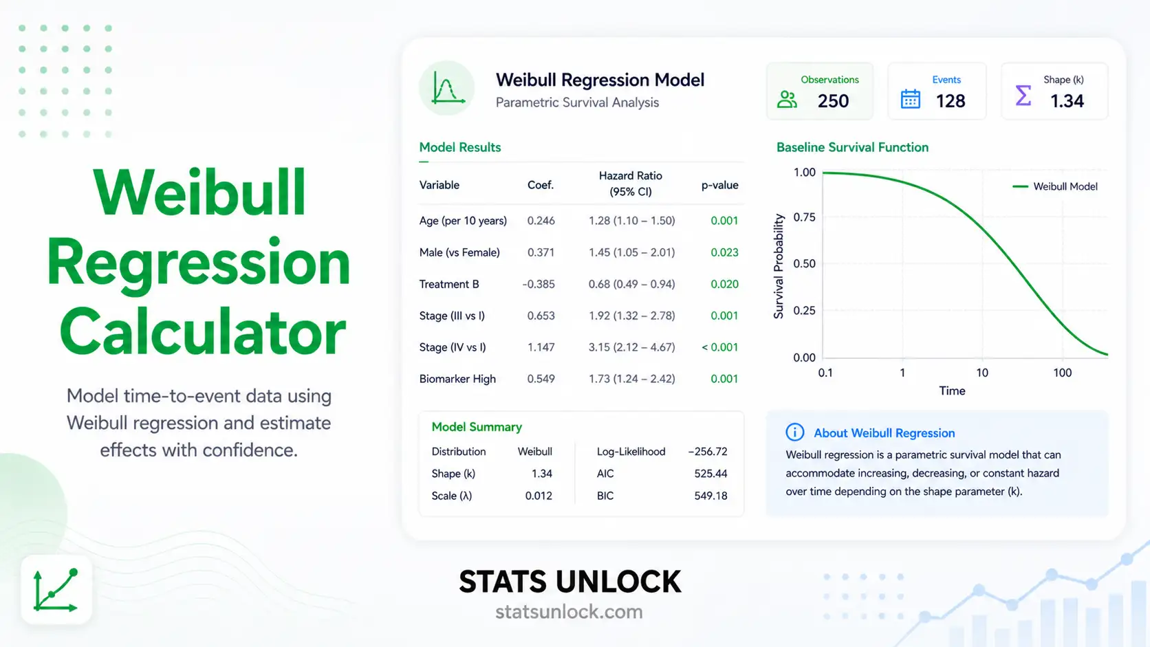
Key Statistics
| Parameter | Estimate | Std Error | z-statistic | p-value | 95% CI Lower | 95% CI Upper |
|---|
Group Summary Statistics
Survival Probability at Key Time Points
Estimated probability of surviving beyond each time point — from the fitted Weibull model. S(t) = exp[−(t/λ)k].
Percentile Survival Times
Time by which a given percentage of subjects have experienced the event. Derived by inverting the survival function: tp = λ · [−ln(1−p)]1/k.
Cumulative Hazard H(t)
H(t) = (t/λ)k. Total accumulated risk up to time t. A straight line on log-log confirms Weibull fit.
Effect Size & Significance
Model Fit & Comparison
Full model (with group predictor) vs null model (intercept + shape only). Lower AIC/BIC = better fit. ΔAIC > 2 is meaningful.
| Model | Parameters | Log-Lik | AIC | BIC | ΔAIC vs Null | LR p-value |
|---|
Visualizations
Detailed Interpretation of Results
📌 What Your Results Mean
Run the analysis to see interpretation.
📋 Assumption Checks
How to Write Your Results in Research
Five ready-to-use write-up templates. Click 📋 Copy to copy directly to your clipboard.
Run the analysis above to generate write-up templates with your actual values.
Conclusion
Summary of Findings
Run the analysis to see a detailed conclusion.
How to Use This Calculator
Prepare Your Data
Collect time-to-event data and event status (1 = event occurred, 0 = censored). Each row represents one subject. Example: time=52, status=1 means the event occurred at time 52.
Choose Your Input Method
Type/paste comma-separated times and statuses, upload a CSV/Excel file, or use the manual grid. Sample datasets are available for quick exploration.
Name Your Groups
Edit the group name fields (e.g., "Treatment vs Control", "High Temperature vs Low Temperature"). These names appear in all results and write-up templates.
Set Significance Level
Choose α = 0.05 (standard), 0.01 (strict), or 0.10 (exploratory). This controls the threshold for statistical significance of the group effect (β coefficient).
Click Run Analysis
The tool fits a Weibull AFT model, estimating the shape (k), scale (λ), and regression coefficient (β) via maximum likelihood. Do NOT click before entering data.
Read the Shape Parameter
k < 1 = decreasing hazard (early failures). k = 1 = constant hazard (exponential). k > 1 = increasing hazard (aging/wear). The shape parameter is one of the most biologically meaningful outputs.
Interpret the Time Ratio
exp(β) is the time ratio (TR). TR = 1.5 means Group A survives 50% longer than Group B. TR = 0.7 means Group A experiences the event 30% sooner. TR > 1 is protective; TR < 1 is harmful.
Review the Four Charts
The survival function shows the probability of surviving beyond time t. The hazard function shows instantaneous risk. The PDF shows event timing. The Weibull probability plot confirms whether the Weibull assumption holds (look for a straight line).
Check Assumptions
Review the assumption checklist. Key assumptions: (1) Weibull distribution fits the data. (2) Hazard ratio is proportional between groups (if using PH interpretation). (3) Censoring is non-informative (random). (4) Observations are independent.
Copy Your Write-Up
Use the five write-up templates (APA 7th, Thesis, Plain Language, Abstract, Pre-Registration) with all values auto-filled. Click Copy and paste directly into your manuscript or report.
📌 When to Use Weibull Regression
Use Weibull regression when you have time-to-event (survival) data with right-censoring and you want a fully parametric model that assumes the Weibull distribution.
✅ Use Weibull Regression When:
• Time-to-event data with censored observations
• You need to extrapolate beyond observation period
• The shape parameter k has scientific meaning
• You want to compare AIC/BIC across distributions
• You need smooth survival curve estimates
• Baseline hazard shape matters to your research
❌ Do NOT Use When:
• The Weibull probability plot is strongly curved
• You cannot assume a parametric distribution
• Outcomes are binary (use logistic regression)
• Data is continuous, non-time-based (use OLS)
• No censoring and non-survival outcome
• Very small samples (< 20 events)
🔬 Common Research Examples:
• Clinical trials: time to disease relapse
• Ecology: nest survival, migration timing
• Engineering: machine component failure
• Business: customer churn duration
• Veterinary science: animal lifespan
• Environmental science: pollutant degradation
⚖️ Weibull vs Cox Regression:
• Weibull: parametric, assumes Weibull distribution, better for extrapolation and prediction
• Cox: semi-parametric, no distributional assumption, more flexible
• Use Weibull when: distribution assumption holds, shape parameter is meaningful
• Use Cox when: distribution is unknown or uncertain
🔢 Technical Notes — Formulas Used
The Weibull Regression (AFT parameterization) uses the following formulas. Each is computed sequentially during maximum likelihood estimation.
Frequently Asked Questions
What is Weibull regression?
What is the difference between Weibull regression and Cox regression?
What does the shape parameter k tell me?
How do I interpret the time ratio (TR = exp(β))?
What is censoring and how does it affect Weibull regression?
How do I check if the Weibull distribution is appropriate?
Can I use Weibull regression with multiple predictors?
What is AIC and how do I use it to compare models?
How do I report Weibull regression results in APA format?
What is the scale parameter λ and what does it mean practically?
How many observations do I need for Weibull regression?
What is the difference between the AFT and PH parameterizations of the Weibull model?
References
This Weibull regression calculator is based on parametric survival analysis and accelerated failure time (AFT) modelling methodology established in peer-reviewed literature. Key references for Weibull regression, survival analysis, and AFT models are listed below.
- Weibull, W. (1951). A statistical distribution function of wide applicability. Journal of Applied Mechanics, 18(3), 293–297. https://doi.org/10.1115/1.4010337
- Cox, D. R., & Oakes, D. (1984). Analysis of survival data. Chapman and Hall. https://doi.org/10.1201/9781315137438
- Kalbfleisch, J. D., & Prentice, R. L. (2002). The statistical analysis of failure time data (2nd ed.). Wiley. https://doi.org/10.1002/9781118032985
- Klein, J. P., & Moeschberger, M. L. (2003). Survival analysis: Techniques for censored and truncated data (2nd ed.). Springer. https://doi.org/10.1007/b97377
- Lawless, J. F. (2003). Statistical models and methods for lifetime data (2nd ed.). Wiley. https://doi.org/10.1002/9781118033005
- Collett, D. (2015). Modelling survival data in medical research (3rd ed.). CRC Press. https://doi.org/10.1201/b18041
- Royston, P., & Parmar, M. K. B. (2002). Flexible parametric proportional-hazards and proportional-odds models for censored survival data. Statistics in Medicine, 21(15), 2175–2197. https://doi.org/10.1002/sim.1203
- Akaike, H. (1974). A new look at the statistical model identification. IEEE Transactions on Automatic Control, 19(6), 716–723. https://doi.org/10.1109/TAC.1974.1100705
- Burnham, K. P., & Anderson, D. R. (2002). Model selection and multimodel inference: A practical information-theoretic approach (2nd ed.). Springer. https://doi.org/10.1007/b97636
- Therneau, T. M., & Grambsch, P. M. (2000). Modeling survival data: Extending the Cox model. Springer. https://doi.org/10.1007/978-1-4757-3294-8
- Hosmer, D. W., & Lemeshow, S. (1999). Applied survival analysis: Regression modeling of time to event data. Wiley. https://doi.org/10.1002/9781118884997
- Meeker, W. Q., & Escobar, L. A. (1998). Statistical methods for reliability data. Wiley. https://doi.org/10.1002/9780470316696
- Venables, W. N., & Ripley, B. D. (2002). Modern applied statistics with S (4th ed.). Springer. https://doi.org/10.1007/978-0-387-21706-2
- R Core Team. (2024). R: A language and environment for statistical computing. R Foundation for Statistical Computing. https://www.R-project.org/
- Harrell, F. E. (2015). Regression modeling strategies: With applications to linear models, logistic and ordinal regression, and survival analysis (2nd ed.). Springer. https://doi.org/10.1007/978-3-319-19425-7


