Cox Proportional Hazards Calculator
A free online Cox proportional hazards (Cox PH) regression tool for survival analysis — estimate hazard ratios, p-values, 95% confidence intervals, the concordance index, and adjusted survival curves from your own time-to-event data.
📥 Enter Your Survival Data
Provide three things per subject: the follow-up time, the event status (1 = event occurred, 0 = censored), and one or more covariates. Comma-separated input is the default. You can rename the covariate (group) below.
; in the covariate box (e.g. 0;55, 1;62, 0;48 for group;age). One covariate is the default.📊 Results
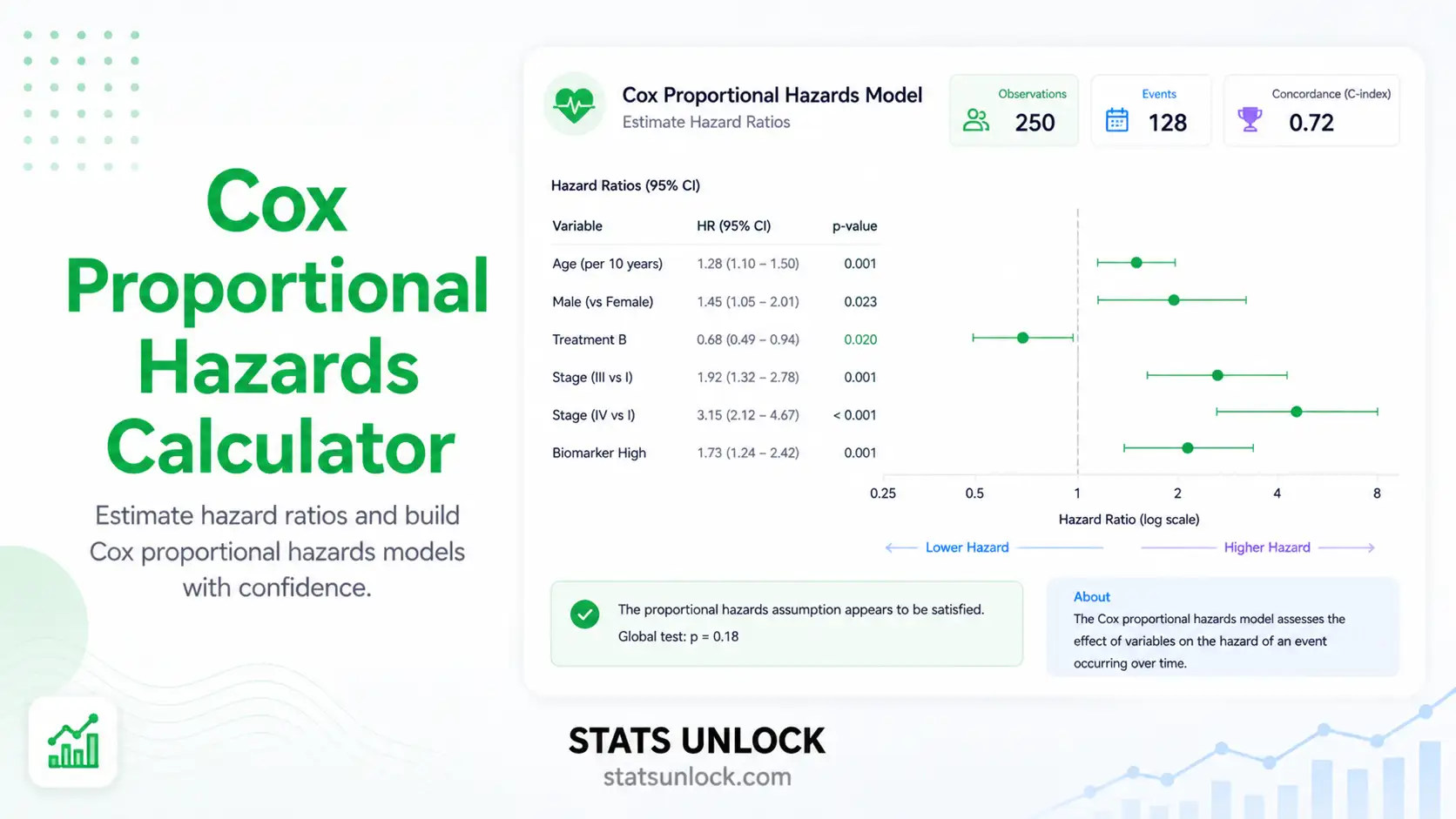
Coefficient Table
Hazard Ratio Details
Model Fit & Global Tests
Baseline & Survival Summary
📈 Visualizations
Three colourful plots summarising the fitted Cox proportional hazards model.
1 · Adjusted Survival Curves by Group
2 · Baseline Cumulative Hazard
3 · Schoenfeld Residuals vs Time (PH check)
⬇️ Export Results
🧪 Assumption Checks
💡 Interpretation of Results
✍️ How to Write Your Results in Research (5 Templates)
📐 Technical Notes & Formulas
A. Formulas Used
B. Technical Notes
- The Cox model is semi-parametric: it estimates covariate effects (β) without assuming any shape for the baseline hazard h0(t).
- Coefficients are estimated by maximising the partial likelihood, which conditions on the observed event times and ignores h0(t).
- Efron's approximation handles tied event times more accurately than Breslow's and is the default here.
- Standard errors come from the inverse observed information matrix; p-values use the Wald z-test.
- If the PH assumption fails for a covariate, consider stratification, time-varying covariates, or an accelerated failure time (AFT) model instead.
🎯 When to Use the Cox Proportional Hazards Model
This free Cox proportional hazards tool is designed for any study where the outcome is the time until an event and you want to measure how predictors change the risk of that event over time, while handling censored observations.
Decision Checklist
- Your outcome is a time-to-event (survival time, time to failure, time to churn)
- Some observations are censored (the event had not happened by study end)
- You want hazard ratios for one or more predictors (continuous or categorical)
- You can reasonably assume the hazard ratio is constant over time (proportional hazards)
- Do NOT use if you only need to compare survival curves between 2–3 groups → use Kaplan-Meier + log-rank test
- Do NOT use if the proportional hazards assumption is clearly violated → use time-varying Cox, stratified Cox, or an AFT (Weibull) model
- Do NOT use if your outcome is a simple binary yes/no with no timing → use logistic regression
Real-World Examples
🏥 Medical Research
Does a new chemotherapy regimen lower the hazard of relapse compared with standard care, adjusting for tumour stage and age?
⚙️ Engineering / Reliability
How does operating load affect the hazard of mechanical failure in turbines, accounting for units still running at study end?
📈 Business / Customer Analytics
Which subscription plan is associated with a higher hazard of customer churn over the first 24 months?
🦅 Ecology / Wildlife
Does GPS-collar transmitter weight influence the hazard of tag failure or animal mortality in a radio-telemetry study with right-censored tracking?
Sample Size Guidance
A practical rule of thumb is 10–15 events per predictor (events, not subjects). With 3 covariates you would aim for roughly 30–45 events. Few events give unstable hazard ratios and very wide confidence intervals.
Related Methods — Decision Tree
📘 How to Use This Cox PH Calculator — Step by Step
Worked example: a cancer trial comparing a treatment group (coded 1) against a control group (coded 0), with survival time in months.
- Enter your data Paste three aligned columns — Time, Event (1/0), and Covariate. Example time row:
52, 48, 55, 61, 47, ... - Choose a sample dataset Pick any of the five built-in datasets from the dropdown to see the tool work instantly; dataset 1 (Cancer Trial) is pre-loaded.
- Name your covariate Type a meaningful name like
treatmentordosein the editable group-name box so every result is labelled clearly. - Configure settings Set the significance level (α = 0.05 → 95% CI), choose Efron tie handling, and leave iterations at 50.
- Run the analysis Click "Run Cox PH Analysis." The model fits via Newton-Raphson in milliseconds.
- Read the summary cards See the hazard ratio, its p-value, the concordance index, and the number of events at a glance. Green = significant, red = not significant.
- Read the coefficient table Each row shows β, HR = exp(β), SE, z, p, and the 95% CI for the hazard ratio.
- Examine the four plots Adjusted survival curves, the hazard-ratio forest plot, the baseline cumulative hazard, and the Schoenfeld residual plot for the PH check.
- Check assumptions The Schoenfeld trend badge tells you whether the proportional-hazards assumption looks reasonable.
- Export your results Use "Download Doc" for a text report or "Download PDF" for a print-ready document, then copy the ready-made APA sentence into your paper.
❓ Frequently Asked Questions
Q1. What is Cox proportional hazards regression and when should I use it?
Cox proportional hazards regression is a semi-parametric model for time-to-event (survival) data. It estimates how predictors change the hazard — the instantaneous risk of the event — without assuming a specific shape for the baseline hazard. Use it whenever your outcome is the time until an event such as death, relapse, machine failure, or customer churn and some observations are censored.
Q2. What is a hazard ratio (HR) and how do I interpret it?
A hazard ratio is the exponentiated Cox coefficient, exp(β). HR = 1 means no effect, HR > 1 means a higher hazard (worse survival) per one-unit increase in the predictor, and HR < 1 means a lower hazard (better survival). For example, HR = 0.21 means the hazard is about 79% lower for that group.
Q3. What does the p-value mean in a Cox model?
The p-value tests whether a predictor's coefficient differs from zero (equivalently, whether HR differs from 1). A small p-value (for example p < 0.05) suggests the predictor is significantly associated with the hazard. It is the probability of seeing a coefficient this large or larger if the predictor truly had no effect on the hazard.
Q4. What is the proportional hazards assumption?
It states that the hazard ratio between any two individuals stays constant over time. You can check it with Schoenfeld residuals: if they show no trend against time, the assumption holds. A clear upward or downward trend means the effect changes over time, and you may need time-varying covariates or a stratified model.
Q5. What is the concordance index (C-index)?
The concordance index (Harrell's C) measures how well the model ranks survival times — the probability that, for a random pair of subjects, the one who experiences the event sooner had the higher predicted risk. It ranges from 0.5 (chance) to 1.0 (perfect). Values above 0.7 indicate good discrimination.
Q6. What is censoring and how do I code it?
Censoring happens when the event has not occurred by the end of follow-up or the subject is lost to follow-up. Those subjects still tell us they survived at least that long. In this calculator, code an event row as event = 1 and a censored row as event = 0.
Q7. How large a sample do I need for Cox regression?
A widely used rule is at least 10 to 15 events (not just subjects) per predictor. With fewer events the hazard ratio estimates become unstable and the confidence intervals very wide, so always prioritise the number of events over the total sample size.
Q8. What is the difference between Cox regression and Kaplan-Meier?
Kaplan-Meier estimates the survival curve for one or a few groups, and the log-rank test compares them. Cox regression models the effect of continuous and multiple predictors at once and produces adjusted hazard ratios that control for other variables. Use Kaplan-Meier to describe and Cox to model.
Q9. How do I report Cox PH results in APA format?
Report the hazard ratio, its 95% confidence interval, and the p-value — for example: "Treatment was associated with a significantly lower hazard of death, HR = 0.21, 95% CI [0.06, 0.67], p = .008." Always state the number of events and the predictors in the model. See the five reporting templates on this page for full examples.
Q10. Can I use this calculator for published research or assignments?
This tool is built for learning, teaching, and exploratory analysis. For formal publication, confirm the results in peer-reviewed software such as R (survival or lifelines), Python (lifelines), SPSS, SAS, or Stata. Cite as: STATS UNLOCK. (2025). Cox proportional hazards calculator. Retrieved from https://statsunlock.com.
🏁 Conclusion
The Cox proportional hazards model is one of the most widely used tools in survival analysis because it answers a question that simple group comparisons cannot: how does each predictor change the risk of an event over time, while holding the other predictors constant? This Cox proportional hazards calculator brings that full workflow into your browser — you paste or upload your data, click Run, and get hazard ratios, confidence intervals, p-values, a concordance index, baseline cumulative hazard, adjusted survival curves, and a Schoenfeld-residual check for the proportional hazards assumption, all without installing R, Python, SPSS, SAS, or Stata.
The strength of the Cox PH model is its semi-parametric design. It estimates the effect of your covariates through the partial likelihood without forcing the baseline hazard into a fixed shape such as exponential or Weibull. That makes it robust and general: the same model works for clinical trial survival, machine reliability, customer churn, and wildlife or ecological time-to-event data. The output you care about most — the hazard ratio — has a clean reading. HR = 1 means no effect, HR above 1 means higher risk per unit of the predictor, and HR below 1 means a protective effect. The 95% confidence interval tells you how precise that estimate is, and the p-value tells you whether it is distinguishable from "no effect."
Sound conclusions still depend on meeting the model's assumptions. Always confirm that the proportional hazards assumption holds (the Schoenfeld residuals on this page should show no trend against time), that you have enough events — roughly 10 to 15 events per predictor — and that censoring is non-informative. When the proportional hazards assumption fails, consider a stratified Cox model, time-varying covariates, or an accelerated failure time model instead. Treat a borderline or violated assumption as a signal to refine the model, not as a reason to discard the analysis.
In short, use this calculator to learn the method, explore your data, and draft your results quickly with the built-in APA, thesis, and plain-language templates. For a final publication, reproduce the fit in peer-reviewed software and cite both the original methodology and your software. Used this way, the Cox proportional hazards model turns censored, messy time-to-event data into a clear, defensible statement about what drives risk — and that is exactly what good survival analysis should deliver.
📚 References
The following references support the statistical methods used in this Cox proportional hazards calculator, covering survival analysis, hazard ratio estimation, and best practices in proportional hazards regression and reporting.
- Cox, D. R. (1972). Regression models and life-tables. Journal of the Royal Statistical Society: Series B, 34(2), 187–202. https://doi.org/10.1111/j.2517-6161.1972.tb00899.x
- Cox, D. R. (1975). Partial likelihood. Biometrika, 62(2), 269–276. https://doi.org/10.1093/biomet/62.2.269
- Efron, B. (1977). The efficiency of Cox's likelihood function for censored data. Journal of the American Statistical Association, 72(359), 557–565. https://doi.org/10.1080/01621459.1977.10480613
- Breslow, N. (1974). Covariance analysis of censored survival data. Biometrics, 30(1), 89–99. https://doi.org/10.2307/2529620
- Schoenfeld, D. (1982). Partial residuals for the proportional hazards regression model. Biometrika, 69(1), 239–241. https://doi.org/10.1093/biomet/69.1.239
- Grambsch, P. M., & Therneau, T. M. (1994). Proportional hazards tests and diagnostics based on weighted residuals. Biometrika, 81(3), 515–526. https://doi.org/10.1093/biomet/81.3.515
- Harrell, F. E., Lee, K. L., & Mark, D. B. (1996). Multivariable prognostic models. Statistics in Medicine, 15(4), 361–387. https://doi.org/10.1002/(SICI)1097-0258(19960229)15:4<361::AID-SIM168>3.0.CO;2-4
- Therneau, T. M., & Grambsch, P. M. (2000). Modeling survival data: Extending the Cox model. Springer. https://doi.org/10.1007/978-1-4757-3294-8
- Bradburn, M. J., Clark, T. G., Love, S. B., & Altman, D. G. (2003). Survival analysis part II: Multivariate data analysis. British Journal of Cancer, 89(3), 431–436. https://doi.org/10.1038/sj.bjc.6601119
- Vittinghoff, E., & McCulloch, C. E. (2007). Relaxing the rule of ten events per variable in logistic and Cox regression. American Journal of Epidemiology, 165(6), 710–718. https://doi.org/10.1093/aje/kwk052
- Spruance, S. L., Reid, J. E., Grace, M., & Samore, M. (2004). Hazard ratio in clinical trials. Antimicrobial Agents and Chemotherapy, 48(8), 2787–2792. https://doi.org/10.1128/AAC.48.8.2787-2792.2004
- Davidson-Pilon, C. (2019). lifelines: Survival analysis in Python. Journal of Open Source Software, 4(40), 1317. https://doi.org/10.21105/joss.01317
- Therneau, T. M. (2024). A package for survival analysis in R (survival package). R Foundation. https://cran.r-project.org/package=survival
- Clark, T. G., Bradburn, M. J., Love, S. B., & Altman, D. G. (2003). Survival analysis part I: Basic concepts and first analyses. British Journal of Cancer, 89(2), 232–238. https://doi.org/10.1038/sj.bjc.6601118
- American Psychological Association. (2020). Publication manual of the American Psychological Association (7th ed.). APA. https://doi.org/10.1037/0000165-000


