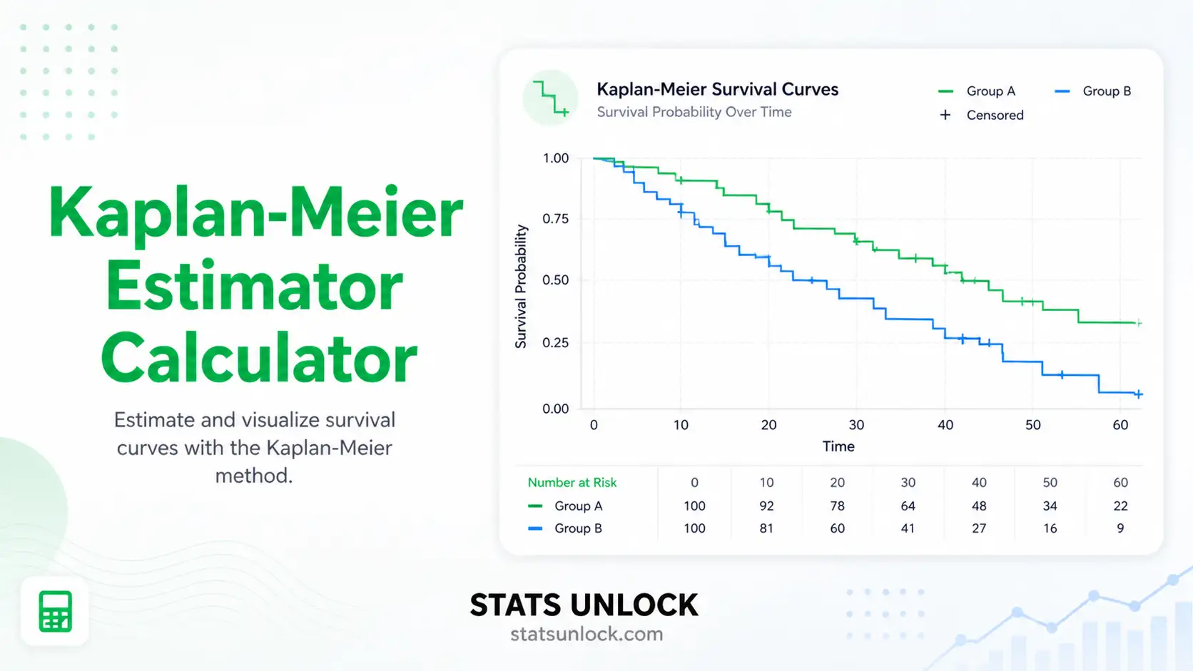
Kaplan-Meier Estimator Calculator
Estimate the survival function from time-to-event data with right-censored observations. Compare groups with the log-rank test, get Greenwood 95% confidence intervals, median survival, and publication-ready APA results — all in one place.
📥 Step 1 — Enter Your Survival Data
Each subject needs two values: time (when they were last observed) and event status (1 = event happened, e.g. death/failure; 0 = censored). Add as many groups (clusters) as you want and rename them to match your study.
.csv, .txt, .xlsx, .xls — click each
numeric column you want loaded as a separate cluster.
⚙️ Step 2 — Configure the Analysis
Adjust significance level, confidence interval method, and time-point reporting.
Computes survival function, Greenwood CIs, median survival, and log-rank test.
📚 When to Use the Kaplan-Meier Estimator
The free Kaplan-Meier estimator calculator on this page is built for clinical researchers, epidemiologists, biostatisticians, ecologists, reliability engineers, and graduate students working with time-to-event data. The tool implements the Kaplan & Meier (1958) non-parametric product-limit estimator, the standard method for estimating survival probability when observations may be right-censored.
Use this method when:
- Your outcome is the time until an event (death, failure, relapse, churn, dispersal).
- Some subjects are right-censored — they exited the study before the event occurred.
- You want a non-parametric estimate that makes no distributional assumption about survival times.
- You need to compare survival between two or more independent groups.
- You want a step-function survival curve and median survival time, not a parametric model.
Real-world examples:
- Oncology: Time from diagnosis to death, comparing chemotherapy regimens.
- Cardiology: Time to first myocardial infarction in trial arms.
- Engineering: Hours until light-bulb / bearing / battery failure across vendors.
- Marketing: Days until a customer cancels their subscription.
- Wildlife ecology: Days a radio-collared animal survives in different habitats.
- Public health: Months from HIV diagnosis to AIDS-defining illness.
Decision tree — pick the right analysis:
🔬 Technical Notes — Formulas & Assumptions
1. Kaplan-Meier (Product-Limit) Estimator
- tj
- = distinct event time (j-th).
- dj
- = number of events at tj.
- nj
- = number at risk just before tj.
2. Greenwood's Variance
Standard error = √Var[Ŝ(t)]. The complementary log-log transform keeps 95% CIs within [0, 1].
3. Complementary log-log 95% CI
where σ̂ = SE[Ŝ(t)] / [Ŝ(t) · ln Ŝ(t)] and z = 1.96 for α = 0.05.
4. Cumulative Hazard (Nelson-Aalen-style from KM)
5. Log-Rank Test Statistic (k groups)
df = k − 1. Oi = observed events in group i; Ei = expected events under H₀ (all groups identical).
Key Assumptions
- Non-informative censoring: censored subjects have the same future risk as those still under observation.
- No calendar-time effect: survival probability does not change because a subject entered the study earlier or later.
- Independent observations: events in one subject do not affect events in another.
- Proportional hazards (for log-rank only): hazard ratio between groups stays roughly constant over time. Crossing curves violate this.
🛠️ How to Use This Kaplan-Meier Calculator — Step-by-Step
Enter your data
Three input options: Type / Paste, Upload CSV / Excel, or pick a built-in Sample dataset. For each group, paste a comma-separated list of times and a comma-separated list of event indicators (1 = event, 0 = censored). Counts must match.
Rename groups & add clusters
Click any group title to rename it (e.g., "Treatment A", "Forest Habitat"). Use Add Another Group to compare 2, 3, 4, or more groups.
Choose a sample dataset (optional)
Five built-in datasets cover oncology, cardiac surgery, engineering reliability, customer churn, and wildlife telemetry. Dataset 1 is pre-loaded so you can run the analysis immediately.
Configure analysis
Set α (default 0.05). Pick the CI method — complementary log-log is recommended. List the time-points where you want survival probability reported (e.g., 6, 12, 24).
Run the analysis
Click Run Kaplan-Meier Analysis. Summary cards appear with median survival, total events, and the log-rank p-value when ≥ 2 groups are present.
Read the four visualizations
① KM step curve (the answer to "how does survival drop over time?"); ② Cumulative hazard (linearises the curve to spot constant-vs-changing hazard); ③ 95% CI bands (uncertainty around the curve); ④ Number-at-risk bars (sample size per time bin — judge how much to trust the tail).
Inspect the group table
Per group: n, events, censored, median survival with 95% CI, and survival probability at each of your requested time-points. Bold green = group with longest median; orange = "not reached".
Read the log-rank test
χ² with k − 1 degrees of freedom. p < α → at least one group differs. Always pair with the plot — if curves cross, the log-rank loses power and you should consider a weighted variant.
Use the interpretation & writing examples
Step 8 explains the result in plain English. Step 9 gives five ready-to-paste reporting formats — APA, thesis, plain-language, abstract, pre-registration. Tap 📋 Copy.
Export the report
Two buttons: Download Doc (plain-text .txt) for editable rough drafts, or Download PDF (full styled report) for sharing and submission.
❓ Frequently Asked Questions
Top 10 questions about Kaplan-Meier survival analysis.
Q1. What is the Kaplan-Meier estimator and when should I use it?
The Kaplan-Meier (KM) estimator, introduced by Kaplan and Meier in 1958, is a non-parametric method that estimates the survival function S(t) — the probability of surviving beyond time t. It is the right tool when your outcome is the time until an event of interest (death, machine failure, relapse, customer churn) and some observations are right-censored (the event had not happened by the time the subject left the study).
Use Kaplan-Meier whenever you want a curve that makes no distributional assumption and an estimate of median survival time. Pair it with the log-rank test to compare two or more groups.
Q2. What does censoring mean and how does Kaplan-Meier handle it?
A subject is right-censored when we know they had not yet experienced the event by some time c, but we do not know what happened afterwards. Common reasons: the study ended, the patient was lost to follow-up, or the equipment was withdrawn.
Kaplan-Meier accounts for censoring by removing each censored subject from the risk-set at their censoring time without counting them as an event. This keeps the survival probability mathematically unbiased so long as the censoring is non-informative.
Q3. How is median survival time computed?
The median survival is the smallest time t at which the estimated survival probability Ŝ(t) drops to 0.50 or below. If the curve plateaus above 0.50 (because too many subjects were censored before half had the event), the median is reported as "not reached". The 95% confidence interval for the median is found by inverting the Greenwood-based confidence band — the lower limit is the smallest t where the upper CI of Ŝ(t) drops below 0.50, and the upper limit is the smallest t where the lower CI drops below 0.50.
Q4. What is the log-rank test and how do I interpret its p-value?
The log-rank test is a chi-square test that compares observed events in each group with expected events under the null hypothesis that all groups have identical survival. A small p-value (e.g., p < 0.05) means the curves differ more than chance alone would explain.
The log-rank is most powerful when the hazards are proportional — i.e., the ratio of the two hazards stays roughly constant over time. When curves cross, switch to a weighted log-rank (Peto-Peto, Tarone-Ware) or to restricted mean survival time (RMST).
Q5. What sample size do I need?
Power for survival analysis is driven by the number of events, not the total sample size. A common rule of thumb is at least 30-50 events per group for stable curve estimates. For an 80%-powered log-rank test detecting a hazard ratio of 1.5 between two equally sized groups, you typically need around 250 total events.
If most subjects are censored early, you may need a much larger n to reach the same number of events.
Q6. Can I compare more than two groups?
Yes. The log-rank test extends to k groups using a chi-square statistic with k − 1 degrees of freedom. This calculator accepts any number of groups; just add them with the Add Another Group button. If the overall test is significant, run pairwise log-rank tests with a Bonferroni or Holm correction to identify which groups differ.
Q7. What's the difference between Kaplan-Meier and Cox regression?
Kaplan-Meier is non-parametric and univariate — it describes survival as a function of time only and compares groups via the log-rank test. Cox proportional-hazards regression is semi-parametric and multivariable — it estimates how multiple covariates (continuous and categorical) shift the hazard, returning hazard ratios.
Use Kaplan-Meier first to visualise the data, then move to Cox if you need to adjust for confounders.
Q8. What if my survival curves cross?
Crossing curves violate the proportional-hazards assumption underlying the log-rank test. The standard log-rank loses power and may even fail to detect a real difference. Better choices when curves cross:
• Weighted log-rank (Peto-Peto, Tarone-Ware) — weights early or late events differently.
• Restricted mean survival time (RMST) — compares the area under each curve up to a chosen horizon.
• Time-dependent Cox model — allows the hazard ratio itself to change over time.
Q9. How do I report Kaplan-Meier results in APA 7th edition?
Report per group: n, number of events, censored count, median survival with 95% CI, and survival probability at the key time-points. For the comparison: log-rank χ²(df) = value, p = exact p. Always include the KM plot. Step 9 of this tool auto-fills five publication-ready reporting formats — APA, thesis, plain-language brief, conference abstract, and open-science pre-registration.
Q10. What if my log-rank result is non-significant?
A non-significant p-value (p > α) is not proof that survival is identical across groups. It only means the data did not provide sufficient evidence to reject the null hypothesis. Possible reasons:
• Low power — too few events. Re-check the number of events; a study with n = 200 but only 12 deaths is severely under-powered.
• Crossing hazards — the test cannot detect time-varying differences. Try weighted log-rank or RMST.
• Truly small effect — the curves really may be similar. Report the effect estimate (median ratio, HR estimate from Cox)
with its CI to quantify how small the true difference might be.
📚 References
The Kaplan-Meier estimator calculator on this page is grounded in these peer-reviewed sources on survival analysis, log-rank testing, and Greenwood confidence intervals. Click each title to access the original publication.
- Kaplan, E. L., & Meier, P. (1958). Nonparametric estimation from incomplete observations. Journal of the American Statistical Association, 53(282), 457–481. https://doi.org/10.1080/01621459.1958.10501452
- Greenwood, M. (1926). The natural duration of cancer. Reports on Public Health and Medical Subjects, 33, 1–26. Her Majesty's Stationery Office. (Foundational source for the Greenwood variance formula.)
- Mantel, N. (1966). Evaluation of survival data and two new rank order statistics arising in its consideration. Cancer Chemotherapy Reports, 50(3), 163–170. https://pubmed.ncbi.nlm.nih.gov/5910392/
- Peto, R., & Peto, J. (1972). Asymptotically efficient rank invariant test procedures. Journal of the Royal Statistical Society: Series A, 135(2), 185–207. https://doi.org/10.2307/2344317
- Cox, D. R. (1972). Regression models and life-tables. Journal of the Royal Statistical Society: Series B, 34(2), 187–220. https://doi.org/10.1111/j.2517-6161.1972.tb00899.x
- Klein, J. P., & Moeschberger, M. L. (2003). Survival Analysis: Techniques for Censored and Truncated Data (2nd ed.). Springer. https://doi.org/10.1007/b97377
- Collett, D. (2015). Modelling Survival Data in Medical Research (3rd ed.). Chapman and Hall/CRC. https://doi.org/10.1201/b18041
- Therneau, T. M., & Grambsch, P. M. (2000). Modeling Survival Data: Extending the Cox Model. Springer. https://doi.org/10.1007/978-1-4757-3294-8
- Bland, J. M., & Altman, D. G. (1998). Survival probabilities (the Kaplan-Meier method). BMJ, 317(7172), 1572. https://doi.org/10.1136/bmj.317.7172.1572
- Rich, J. T., Neely, J. G., Paniello, R. C., et al. (2010). A practical guide to understanding Kaplan-Meier curves. Otolaryngology–Head and Neck Surgery, 143(3), 331–336. https://doi.org/10.1016/j.otohns.2010.05.007
- Royston, P., & Parmar, M. K. (2013). Restricted mean survival time: an alternative to the hazard ratio for the design and analysis of randomized trials with a time-to-event outcome. BMC Medical Research Methodology, 13(1), 152. https://doi.org/10.1186/1471-2288-13-152
- Schoenfeld, D. (1981). The asymptotic properties of nonparametric tests for comparing survival distributions. Biometrika, 68(1), 316–319. https://doi.org/10.1093/biomet/68.1.316
- Pocock, S. J., Clayton, T. C., & Altman, D. G. (2002). Survival plots of time-to-event outcomes in clinical trials: good practice and pitfalls. The Lancet, 359(9318), 1686–1689. https://doi.org/10.1016/S0140-6736(02)08594-X
- R Core Team (2024). R: A language and environment for statistical computing. R Foundation for Statistical Computing. https://www.r-project.org/
- Therneau, T. M. (2024). survival: Survival Analysis. R package version 3.5-8. https://cran.r-project.org/package=survival


