How do I interpret an odds ratio in logistic regression?

An odds ratio (OR) above 1 means the predictor increases the odds of the outcome; below 1 means it decreases them. For example, OR = 2.5 means a one-unit increase in X multiplies the odds of the outcome by 2.5.

What is a good AUC value for logistic regression?

AUC ranges from 0.5 (random guess) to 1.0 (perfect classifier). Values above 0.7 indicate acceptable discrimination, above 0.8 is good, and above 0.9 is excellent.

What is the p-value for a logistic regression coefficient?

It is the probability of obtaining a Wald z-statistic as extreme as observed if the true coefficient were zero. p < 0.05 typically indicates the predictor is statistically significant.

What sample size do I need for logistic regression?

A common rule of thumb is at least 10 events per predictor (EPV ≥ 10). For one predictor and a balanced outcome, aim for at least 50–100 observations.

What is pseudo R-squared in logistic regression?

Pseudo R² (McFadden, Cox & Snell, Nagelkerke) approximates the proportion of variance explained. McFadden values of 0.2–0.4 are considered good fit.

How does logistic regression differ from linear regression?

Linear regression predicts continuous outcomes using OLS; logistic regression predicts probabilities for binary outcomes via the logit link, returning values bounded between 0 and 1.

What does the intercept (β₀) mean in logistic regression?

The intercept is the log-odds of the outcome when X = 0. Exponentiating it gives the baseline odds. Centering predictors makes the intercept more interpretable.

Can I use logistic regression with a small sample?

With small samples (n < 50), maximum likelihood estimates can be biased. Consider exact logistic regression or Firth's penalized likelihood as alternatives.

How do I report logistic regression results in APA 7 format?

Report β, SE, Wald z (or χ²), p, OR with 95% CI, and overall model fit (e.g., -2LL, McFadden R²). Example: β = 0.85, SE = 0.21, z = 4.05, p < .001, OR = 2.34, 95% CI [1.55, 3.53].

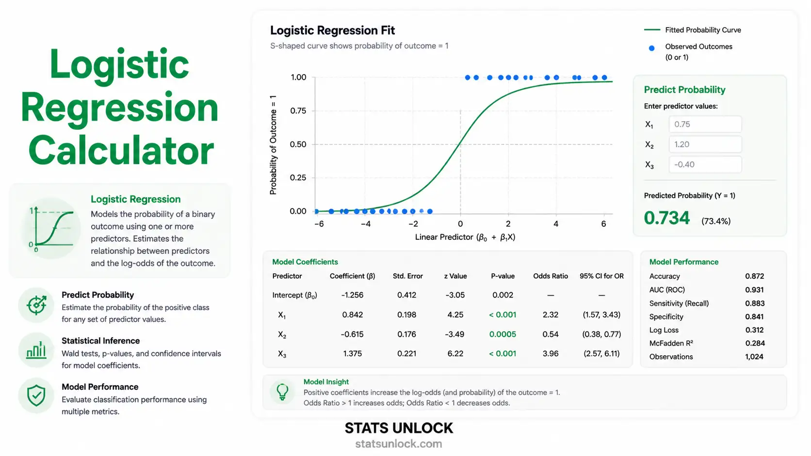
Logistic Regression Calculator (Free, Online) — Binary GLM with Odds Ratio

📊 1. Enter Your Data

Provide your binary outcome (Y) and continuous predictor (X). Use the sample dataset to get started, or paste your own values.

Sample dataset:

Dataset / Group Name (editable):

This name appears in results, charts, and exports.

Predictor (X) — comma-separated

Continuous predictor variable.

Outcome (Y) — binary 0/1, comma-separated

Binary outcome (0 = no/fail; 1 = yes/pass).

Upload CSV or Excel file:

Supports .csv, .txt, .xlsx, .xls — headers detected automatically.

Enter rows of (X, Y) pairs. Y must be 0 or 1.

X (Predictor)	Y (0 or 1)

Alpha Level (α):

Classification Threshold:

Center Predictor (X):

📐 9. Technical Notes & Formulas

Formulas Used

Logistic Model

P(Y=1 | X) = 1 / (1 + exp(−(β₀ + β₁X)))

Where: P(Y=1 | X) = probability that Y = 1 given X β₀ = intercept (log-odds when X = 0) β₁ = slope (change in log-odds per unit X) exp = natural exponential function

Logit Link

logit(p) = ln(p / (1 − p)) = β₀ + β₁X

Where: ln = natural logarithm p / (1−p) = odds of Y = 1 β₀, β₁ = model coefficients

Odds Ratio

OR = exp(β₁) 95% CI for OR = exp(β₁ ± z(α/2) · SE(β₁))

Where: OR = odds ratio for one-unit increase in X z(α/2) = critical z value (1.96 for α = 0.05) SE(β₁) = standard error of the slope

Wald Test

z = β / SE(β) p = 2 · (1 − Φ(|z|))

Where: z = Wald z-statistic Φ = standard normal CDF SE = standard error of the coefficient

Maximum Likelihood & Deviance

LL = Σ [ yᵢ · ln(pᵢ) + (1 − yᵢ) · ln(1 − pᵢ) ] −2LL = deviance McFadden R² = 1 − (LL_full / LL_null) AIC = −2LL + 2k BIC = −2LL + k · ln(n)

Where: LL = log-likelihood yᵢ, pᵢ = observed and predicted values k = number of parameters n = sample size

Classification Metrics

Accuracy = (TP + TN) / N Sensitivity = TP / (TP + FN) Specificity = TN / (TN + FP) Precision = TP / (TP + FP) F1 = 2·(P·R)/(P+R)

Technical Notes

Estimation method: Iteratively Reweighted Least Squares (IRLS / Newton–Raphson) maximizes the binomial log-likelihood. Converges in < 30 iterations on well-conditioned data.

Link function: Logit. Logistic regression is the canonical binomial GLM in the exponential family.

Standard errors: Derived from the inverse of the Fisher information matrix (Hessian).

Coefficient interpretation: A one-unit increase in X multiplies the odds of Y = 1 by exp(β). β > 0 increases probability; β < 0 decreases it.

Quasi-complete separation: If predictions are perfectly 0 or 1, MLE diverges. Use Firth's penalized likelihood as a remedy.

📚 10. When to Use Logistic Regression

Decision checklist, examples, and decision tree

Use logistic regression when:

Your dependent variable is binary (two categories: 0/1, yes/no, success/failure)
You want to estimate the probability of an outcome from one or more predictors
Predictors can be continuous, ordinal, or categorical (dummy-coded)
Observations are independent
Sample is large enough (≥ 10 events per predictor)
Do NOT use for continuous outcomes → use linear regression
Do NOT use for ordered outcomes (3+ levels) → use ordinal logistic regression
Do NOT use for unordered outcomes (3+ levels) → use multinomial logistic regression
Do NOT use for count data → use Poisson or Negative Binomial regression

Real-world examples

Medical: Predicting heart disease (yes/no) from age, cholesterol, and BMI.
Education: Predicting exam pass/fail from study hours and prior GPA.
Marketing: Predicting whether a customer will click an ad given dwell time and previous behavior.
Ecology / Wildlife: Predicting species presence/absence (1/0) from habitat covariates such as canopy cover.
Finance: Predicting loan default given income, credit score, and debt ratio.

Sample-size guidance

Apply the events-per-variable (EPV) rule: at least 10 events of the rarer outcome per predictor. With 1 predictor and roughly balanced classes, aim for n ≥ 50; with 5 predictors, aim for n ≥ 200 with at least 50 events of each class.

Decision tree

Outcome type?
├── Binary (0/1)        → LOGISTIC REGRESSION (this tool)
├── Ordered 3+          → Ordinal logistic regression
├── Unordered 3+        → Multinomial logistic regression
├── Counts              → Poisson / Negative Binomial
├── Continuous          → Linear regression (OLS)
└── Time-to-event       → Cox PH / survival models

📘 11. How to Use This Tool

Step-by-step walkthrough

Step 1 — Enter your data: Use comma-separated input (default tab). Pick a sample dataset, paste your own values, upload a CSV/Excel file, or use the manual entry table. Edit the dataset name to label your run.

Step 2 — Choose a sample: Five pre-loaded datasets cover education, medical, marketing, finance, and ecology contexts. Each populates X (predictor) and Y (binary outcome) automatically.

Step 3 — Configure settings: Pick alpha (0.01, 0.05, 0.10), classification threshold (0.3–0.7), and whether to center X. Centering produces a more interpretable intercept.

Step 4 — Run analysis: Click Run Logistic Regression. The tool fits the model via Newton–Raphson and updates every section.

Step 5 — Read summary cards: The 4 cards show β₁ (slope), the odds ratio, the Wald p-value, and AUC. Green = significant; amber = marginal; red = non-significant.

Step 6 — Inspect tables: Coefficient, model-fit, classification, and confusion-matrix tables give a full picture of estimates, fit, and predictive performance.

Step 7 — Examine the four charts: Logistic curve, ROC curve, probability distribution by class, and residuals vs fitted. Look for separation between classes and an ROC bowed toward the top-left.

Step 8 — Check assumptions: Linearity of the logit, independence, no perfect separation, and adequate sample size (EPV ≥ 10).

Step 9 — Read the interpretation: Plain-English paragraphs translate β, OR, p, and AUC into decisions you can defend.

Step 10 — Export: "Download Doc" gives a .txt summary; "Download PDF" prints a clean A4 report.

❓ 12. Frequently Asked Questions

Q1. What is logistic regression and when should I use it?

Logistic regression is a generalized linear model (GLM) for predicting a binary outcome (0/1) from one or more predictors. Use it when your outcome has two categories — pass/fail, alive/dead, present/absent — and you want both the probability of the event and the effect of each predictor expressed as an odds ratio.

Q2. What is a p-value, and how do I interpret it for logistic regression?

The Wald p-value is the probability of observing a coefficient as extreme as estimated if the true coefficient were zero. p < 0.05 indicates the predictor's relationship with the outcome is unlikely under the null. It is not the probability that the null is true.

Q3. Does statistical significance equal practical importance?

No. With large n, tiny effects can be statistically significant. Always read the odds ratio together with the p-value. An OR of 1.05 may be significant but offer little real-world impact; an OR of 3.0 changes decisions meaningfully.

Q4. How do I interpret the odds ratio?

OR = exp(β). OR = 1 means no effect; OR > 1 means each unit increase in X multiplies the odds of Y = 1 by that amount; OR < 1 means it divides them. OR = 2.0 doubles the odds; OR = 0.5 halves them.

Q5. What assumptions does logistic regression require?

Independence of observations, linearity between continuous predictors and the logit of the outcome, absence of perfect multicollinearity, no perfect separation of classes, and adequate sample size (events per variable ≥ 10). Normality of residuals is not required.

Q6. How large a sample do I need for logistic regression?

The events-per-variable (EPV) rule: aim for at least 10 events of the rarer outcome per predictor. For one predictor with balanced classes, n ≥ 50 is a practical minimum. For five predictors, plan for n ≥ 200 with ≥ 50 events of each class.

Q7. What is AUC and what is a good value?

AUC is the area under the ROC curve — the probability the model ranks a random positive higher than a random negative. 0.5 = chance; 0.7 = acceptable; 0.8 = good; 0.9 = excellent. AUC alone cannot tell you about calibration or threshold choice.

Q8. How do I report logistic regression results in APA 7th edition format?

Report β, SE, Wald z, p, OR with 95% CI, and overall fit. Example: "A logistic regression revealed that hours studied significantly predicted exam pass, β = 1.50, SE = 0.62, z = 2.42, p = .015, OR = 4.48, 95% CI [1.33, 15.07]." See Section 7 for five reporting templates.

Q9. Can I use this calculator for published research?

Yes for exploratory work and teaching. For peer-reviewed publication, cross-check estimates with R (glm()), Python (statsmodels), SPSS, or SAS. Cite as: StatsUnlock. (2025). Logistic regression calculator. https://statsunlock.com/tools/logistic-regression-calculator/.

Q10. What if my result is non-significant — is my hypothesis wrong?

A non-significant p-value (p > α) means the data do not provide enough evidence to reject the null — not that the null is true. Consider statistical power, sample size, and effect size. Report the OR and CI even when p is non-significant; absence of evidence is not evidence of absence.

📖 13. References

20 peer-reviewed and authoritative sources

The following references support the statistical methods used in this logistic regression calculator, covering maximum likelihood estimation, odds ratio interpretation, confidence interval construction, p-value reporting, ROC/AUC analysis, goodness-of-fit testing, and best practices in generalized linear modeling for binary outcomes.

Foundational Theory

Cox, D. R. (1958). The regression analysis of binary sequences. Journal of the Royal Statistical Society: Series B, 20(2), 215–242. https://doi.org/10.1111/j.2517-6161.1958.tb00292.x
Nelder, J. A., & Wedderburn, R. W. M. (1972). Generalized linear models. Journal of the Royal Statistical Society: Series A, 135(3), 370–384. https://doi.org/10.2307/2344614
McFadden, D. (1974). Conditional logit analysis of qualitative choice behavior. In P. Zarembka (Ed.), Frontiers in Econometrics (pp. 105–142). Academic Press.
Berkson, J. (1944). Application of the logistic function to bio-assay. Journal of the American Statistical Association, 39(227), 357–365. https://doi.org/10.1080/01621459.1944.10500699
Wedderburn, R. W. M. (1974). Quasi-likelihood functions, generalized linear models, and the Gauss–Newton method. Biometrika, 61(3), 439–447. https://doi.org/10.1093/biomet/61.3.439

Textbooks & Comprehensive Treatments

Hosmer, D. W., Lemeshow, S., & Sturdivant, R. X. (2013). Applied Logistic Regression (3rd ed.). Wiley. https://doi.org/10.1002/9781118548387
Agresti, A. (2018). An Introduction to Categorical Data Analysis (3rd ed.). Wiley.
McCullagh, P., & Nelder, J. A. (1989). Generalized Linear Models (2nd ed.). Chapman & Hall/CRC. https://doi.org/10.1201/9780203753736
Harrell, F. E. (2015). Regression Modeling Strategies: With Applications to Linear Models, Logistic and Ordinal Regression, and Survival Analysis (2nd ed.). Springer. https://doi.org/10.1007/978-3-319-19425-7

Sample Size, Bias & Separation

Peduzzi, P., Concato, J., Kemper, E., Holford, T. R., & Feinstein, A. R. (1996). A simulation study of the number of events per variable in logistic regression analysis. Journal of Clinical Epidemiology, 49(12), 1373–1379. https://doi.org/10.1016/S0895-4356(96)00236-3
Firth, D. (1993). Bias reduction of maximum likelihood estimates. Biometrika, 80(1), 27–38. https://doi.org/10.1093/biomet/80.1.27
Heinze, G., & Schemper, M. (2002). A solution to the problem of separation in logistic regression. Statistics in Medicine, 21(16), 2409–2419. https://doi.org/10.1002/sim.1047
Riley, R. D., Snell, K. I. E., Ensor, J., Burke, D. L., Harrell, F. E., Moons, K. G. M., & Collins, G. S. (2019). Minimum sample size for developing a multivariable prediction model: PART II — binary and time-to-event outcomes. Statistics in Medicine, 38(7), 1276–1296. https://doi.org/10.1002/sim.7992

Goodness of Fit, ROC & Calibration

Hosmer, D. W., & Lemeshow, S. (1980). Goodness of fit tests for the multiple logistic regression model. Communications in Statistics — Theory and Methods, 9(10), 1043–1069. https://doi.org/10.1080/03610928008827941
Hanley, J. A., & McNeil, B. J. (1982). The meaning and use of the area under a receiver operating characteristic (ROC) curve. Radiology, 143(1), 29–36. https://doi.org/10.1148/radiology.143.1.7063747
DeLong, E. R., DeLong, D. M., & Clarke-Pearson, D. L. (1988). Comparing the areas under two or more correlated receiver operating characteristic curves: A nonparametric approach. Biometrics, 44(3), 837–845. https://doi.org/10.2307/2531595
Steyerberg, E. W., Vickers, A. J., Cook, N. R., Gerds, T., Gonen, M., Obuchowski, N., Pencina, M. J., & Kattan, M. W. (2010). Assessing the performance of prediction models: A framework for traditional and novel measures. Epidemiology, 21(1), 128–138. https://doi.org/10.1097/EDE.0b013e3181c30fb2
Nagelkerke, N. J. D. (1991). A note on a general definition of the coefficient of determination. Biometrika, 78(3), 691–692. https://doi.org/10.1093/biomet/78.3.691

Reporting Standards & Software

Collins, G. S., Reitsma, J. B., Altman, D. G., & Moons, K. G. M. (2015). Transparent reporting of a multivariable prediction model for individual prognosis or diagnosis (TRIPOD): The TRIPOD statement. BMJ, 350, g7594. https://doi.org/10.1136/bmj.g7594
American Psychological Association. (2020). Publication Manual of the American Psychological Association (7th ed.). APA. https://doi.org/10.1037/0000165-000
R Core Team. (2024). R: A language and environment for statistical computing. R Foundation for Statistical Computing. https://www.R-project.org/
NIST/SEMATECH. (2013). e-Handbook of Statistical Methods. https://www.itl.nist.gov/div898/handbook/

This Tool

StatsUnlock. (2025). Logistic regression calculator. Retrieved from https://statsunlock.com/tools/logistic-regression-calculator/

How to cite this tool (APA 7):
StatsUnlock. (2025). Logistic regression calculator [Online statistical tool]. https://statsunlock.com/tools/logistic-regression-calculator/