What is an odds ratio in ordinal logistic regression?

The odds ratio is exp(beta). It tells you how the odds of being in a higher outcome category multiply for each one unit increase in the predictor, and this multiplier is assumed to be the same across every category cut point under the proportional odds assumption.

How do I interpret the thresholds or cut points?

Each threshold marks the point on the logit scale that separates one cumulative category from the next. Together with the slope they convert any predictor value into the probability of each ordered category.

What does the p-value mean here?

The p-value is the probability of seeing a slope at least this far from zero if the predictor truly had no effect on the ordered outcome. A small p-value (below your alpha) is evidence the predictor genuinely shifts the outcome up or down the order.

What pseudo R-squared values are reported?

The tool reports McFadden, Cox and Snell, and Nagelkerke pseudo R-squared. They are not the same as ordinary R-squared; McFadden values between 0.2 and 0.4 already indicate a very good fit.

How is ordinal regression different from linear regression?

Linear regression predicts a continuous number and assumes equal spacing. Ordinal logistic regression predicts the probability of ordered categories and respects the rank order without assuming the categories are equally spaced.

Can I use this calculator for my thesis or published research?

It is built for learning and exploratory analysis. For formal publication, confirm the results in R (MASS::polr or ordinal::clm), Python (statsmodels OrderedModel), SPSS or SAS, and report the software used.

Ordinal Logistic Regression Calculator – Free Online Proportional Odds Model | StatsUnlock

Ordinal Logistic Regression Calculator – Free Online Proportional Odds Model Tool

Ordinal Logistic Regression Calculator

Fit a proportional odds model to an ordered categorical outcome. Get coefficients, odds ratios, p-values, pseudo R-squared, four colorful charts, and ready-to-paste APA results — free and online.

GLMProportional Odds Ordered LogitFree OnlineAPA Output

📥 Data Input

Each ordered category is one column / cluster. Enter the predictor values (comma-separated) for the subjects in that category. Categories must be listed from lowest to highest. Group names are editable.

Load a sample dataset

Upload CSV or Excel file

Supports .csv, .txt, .xlsx, .xls — headers detected automatically. Click the columns that should each become a category/cluster — every selected column is loaded as a separate ordered category (left to right = lowest to highest).

Use the dropdown on the Paste / Type tab to load any of the 5 built-in datasets, then edit the values or category names directly. The first dataset is pre-loaded so the calculator is ready to run immediately.

⚙️ Model Settings

Predictor name (X)

Significance level (α)

Confidence level

📊 Results

Coefficient Table

Model Fit

Group Descriptive Statistics

Summary of the predictor within each ordered category.

Predicted Probabilities at Key Predictor Values

Model-implied probability of each category across the observed range of the predictor.

Odds Ratios for Common Increments

How the odds of a higher category scale for larger changes in the predictor.

Classification Table

Each observation is assigned to its most probable category. Rows = actual, columns = predicted.

📈 Visualizations

Four colorful views of the fitted proportional odds model.

1 · Predicted Category Probabilities

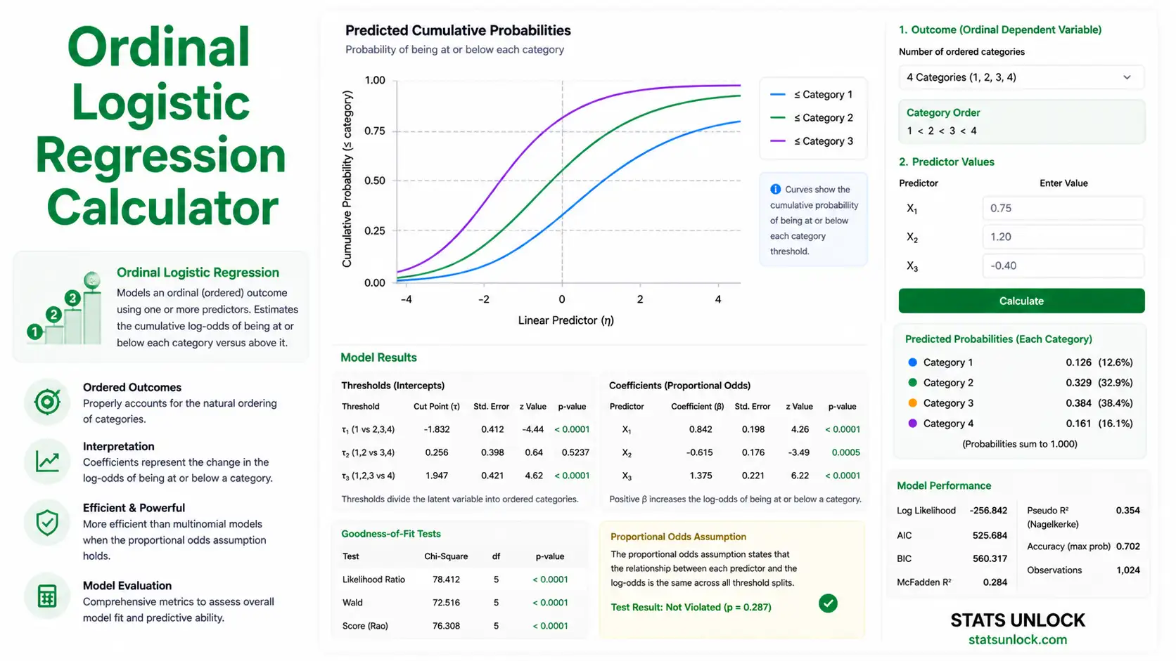
2 · Cumulative Probability Curves

3 · Predictor Distribution by Category

4 · Odds Ratio with 95% CI

🧠 Interpretation of Results

✍️ How to Write Your Results in Research

🔎 Assumption Checks

📐 Technical Notes & Formulas

Formulas Used

Proportional odds (cumulative logit) model: logit[ P(Y ≤ j | x) ] = θⱼ − β·x for j = 1 … J−1 P(Y ≤ j | x) = 1 / (1 + e^−(θⱼ − β·x)) P(Y = j | x) = P(Y ≤ j | x) − P(Y ≤ j−1 | x) Odds ratio: OR = e^β Log-likelihood: ℓ = Σ log P(Y = yᵢ | xᵢ) Wald test: z = β / SE(β), p = 2·[1 − Φ(|z|)] Likelihood ratio: LR = 2(ℓ_full − ℓ_null) ~ χ²(p) McFadden R²: 1 − ℓ_full / ℓ_null Where: Y = ordered outcome category (1 … J, low → high) x = predictor value for a subject θⱼ = j-th threshold / cut point (logit scale) β = common slope (shared across all thresholds) J = number of ordered categories Φ = standard normal CDF ℓ_null = log-likelihood of the intercept-only model

Technical Notes

🎯 When to Use Ordinal Logistic Regression

This free ordinal logistic regression tool is designed for outcomes that have a natural order but unequal or unknown spacing — satisfaction ratings, severity stages, quality grades, Likert items, or league tiers — predicted from one numeric variable.

Your outcome has 3 or more ordered categories (low → high)
The order is meaningful but the gaps between levels are not necessarily equal
Observations are independent of one another
The effect of the predictor is roughly the same across category cut points (proportional odds)
Categories have no order (e.g., colour, brand) → use Multinomial Logistic Regression
Outcome is binary (only two categories) → use Binary Logistic Regression
Outcome is a continuous number with equal spacing → use Linear Regression
Proportional odds clearly fails → use a Partial Proportional Odds or Multinomial model

Real-World Examples

Medicine: predicting pain relief (None / Mild / Moderate / Strong) from drug dose.

Education: predicting grade band (Fail / Pass / Distinction) from study hours.

Ecology & Wildlife: predicting habitat quality class (Poor / Fair / Good) from an NDVI greenness score.

Business: predicting customer tier (Bronze / Silver / Gold) from annual spend.

Decision Tree

Ordered outcome? ── No ──▶ Multinomial logistic regression │ Yes │ 3+ levels? ── No (2 levels) ──▶ Binary logistic regression │ Yes │ Proportional odds holds? ── No ──▶ Partial proportional odds / multinomial │ Yes ──▶ THIS TOOL (Ordinal logistic / proportional odds)

📖 How to Use This Ordinal Logistic Regression Calculator

Step 1 — Enter your data. On the Paste / Type tab, each box is one ordered category. Type the predictor values for that category, comma-separated (e.g., 52, 48, 55, 61, 47). List categories from lowest to highest.

Step 2 — Choose a sample dataset. Pick any of the five built-in examples to see the expected format; dataset 1 is pre-loaded.

Step 3 — Name things. Edit each category name (e.g., Low / Medium / High) and set the predictor name (e.g., Score). Names flow through to every chart and report.

Step 4 — Configure. Pick the significance level α (0.05 is standard). The confidence level updates automatically.

Step 5 — Run. Click Run Ordinal Logistic Regression. Nothing runs until you click.

Step 6 — Read the summary cards. Green means the predictor is significant at your α; amber means it is not.

Step 7 — Read the coefficient table. The slope β, its odds ratio, z, and p tell you the direction and strength of the effect; thresholds separate the categories.

Step 8 — Examine the four charts. Watch how category probabilities shift as the predictor increases, and check the odds ratio plot against the reference line at 1.

Step 9 — Check assumptions. Review the proportional-odds and sample-size notes before trusting the result.

Step 10 — Export. Download a Word-style .txt report or a print-ready PDF, or copy an APA sentence straight into your manuscript.

❓ Frequently Asked Questions

Q1. What is ordinal logistic regression and when should I use it?

Ordinal logistic regression — the proportional odds model — predicts an ordered categorical outcome (Low → Medium → High) from one or more predictors. Use it when the outcome has a natural rank order but the distances between levels are not equal, such as a 1–5 satisfaction rating or a disease severity stage.

Q2. What is an odds ratio here, and how do I read it?

The odds ratio is exp(β). It is the factor by which the odds of being in a higher category multiply for each one-unit rise in the predictor. OR > 1 means higher predictor values push the outcome up the order; OR < 1 pushes it down; OR = 1 means no effect.

Q3. What is the proportional odds assumption?

It assumes the predictor's effect (the slope β) is the same across every cumulative split of the ordered outcome, so only the thresholds change. If a Brant test or separate cut-point logistic models show very different slopes, the assumption is violated — consider a partial proportional odds or multinomial model.

Q4. What do the thresholds / cut points mean?

Each threshold θⱼ is the point on the logit scale that divides category j from category j+1 when the predictor is zero. Together with the slope they convert any predictor value into the probability of each ordered category. They should always increase in order.

Q5. What does the p-value tell me?

The p-value is the chance of seeing a slope at least this far from zero if the predictor truly had no effect on the ordered outcome. A value below your α is evidence the predictor genuinely shifts the outcome up or down the order. It is not the probability that the null hypothesis is true.

Q6. Which pseudo R-squared should I report?

The tool gives McFadden, Cox & Snell, and Nagelkerke. They are not equivalent to ordinary R². McFadden values of 0.2–0.4 already indicate a very good fit. Nagelkerke rescales Cox & Snell so it can reach 1, making it easier to communicate.

Q7. How large a sample do I need?

A practical rule is at least 10 observations in the smallest outcome category per predictor, and ideally 20+ per category overall. Very small categories make the threshold and slope estimates unstable and inflate standard errors.

Q8. How is this different from linear regression?

Linear regression predicts a continuous number and assumes equal spacing between values. Ordinal logistic regression predicts the probability of each ordered category and respects the rank order without assuming the categories are equally spaced.

Q9. Can I use this for my thesis or a published paper?

It is built for learning and exploratory analysis. For formal publication, confirm the numbers in R (MASS::polr or ordinal::clm), Python (statsmodels OrderedModel), SPSS, or SAS, and cite the software you used. Suggested citation: STATS UNLOCK. (2025). Ordinal logistic regression calculator. https://statsunlock.com.

Q10. What if the slope is non-significant?

A non-significant slope means the data do not give enough evidence that the predictor moves the outcome along its order. It does not prove there is no effect — a larger sample, a better-measured predictor, or a different model may still reveal one. Check whether your study had enough power.

✅ Conclusion

⬇️ Export Your Results

🔗 Copy summary to clipboard

📚 References

The following peer-reviewed references support the methods used in this ordinal logistic regression calculator, covering the proportional odds model, odds ratio interpretation, and best practices in hypothesis testing.

McCullagh, P. (1980). Regression models for ordinal data. Journal of the Royal Statistical Society: Series B, 42(2), 109–142. https://doi.org/10.1111/j.2517-6161.1980.tb01109.x
Brant, R. (1990). Assessing proportionality in the proportional odds model for ordinal logistic regression. Biometrics, 46(4), 1171–1178. https://doi.org/10.2307/2532457
Ananth, C. V., & Kleinbaum, D. G. (1997). Regression models for ordinal responses: A review of methods and applications. International Journal of Epidemiology, 26(6), 1323–1333. https://doi.org/10.1093/ije/26.6.1323
Bender, R., & Grouven, U. (1997). Ordinal logistic regression in medical research. Journal of the Royal College of Physicians of London, 31(5), 546–551. https://doi.org/10.1177/014107689709000601
Agresti, A. (1999). Modelling ordered categorical data: Recent advances and future challenges. Statistics in Medicine, 18(17–18), 2191–2207. https://doi.org/10.1002/(SICI)1097-0258
Williams, R. (2006). Generalized ordered logit / partial proportional odds models for ordinal dependent variables. The Stata Journal, 6(1), 58–82. https://doi.org/10.1177/1536867X0600600104
Fullerton, A. S. (2009). A conceptual framework for ordered logistic regression models. Sociological Methods & Research, 38(2), 306–347. https://doi.org/10.1177/0049124109346162
Liddell, T. M., & Kruschke, J. K. (2018). Analyzing ordinal data with metric models: What could possibly go wrong? Journal of Experimental Social Psychology, 79, 328–348. https://doi.org/10.1016/j.jesp.2018.08.009
Bürkner, P.-C., & Vuorre, M. (2019). Ordinal regression models in psychology: A tutorial. Advances in Methods and Practices in Psychological Science, 2(1), 77–101. https://doi.org/10.1177/2515245918823199
McFadden, D. (1974). Conditional logit analysis of qualitative choice behavior. In P. Zarembka (Ed.), Frontiers in Econometrics (pp. 105–142). Academic Press. https://doi.org/10.1080/01621459.1974.10482955
Nagelkerke, N. J. D. (1991). A note on a general definition of the coefficient of determination. Biometrika, 78(3), 691–692. https://doi.org/10.1093/biomet/78.3.691
Cohen, J. (1992). A power primer. Psychological Bulletin, 112(1), 155–159. https://doi.org/10.1037/0033-2909.112.1.155
Christensen, R. H. B. (2019). Cumulative link models for ordinal regression with the R package ordinal. Journal of Statistical Software. https://doi.org/10.18637/jss.v097.i01
Harrell, F. E. (2015). Regression modeling strategies (2nd ed.). Springer. https://doi.org/10.1007/978-3-319-19425-7
Norris, C. M., Ghali, W. A., Saunders, L. D., et al. (2006). Ordinal regression model and the linear regression model were superior to the logistic regression models. Journal of Clinical Epidemiology, 59(5), 448–456. https://doi.org/10.1016/j.jclinepi.2005.09.007