Gamma Regression Calculator
Fit a generalized linear model for positive, right-skewed continuous outcomes. Get coefficients, deviance, p-values, AIC, dispersion estimates and APA-format results — instantly.
📥 1. Input Your Data
Enter X and Y values one row at a time. Click Add Row for more.
⚙️ 2. Model Configuration
📊 3. Analysis Results
Summary Cards
Coefficient Table
| Term | Estimate (β) | SE | z | p-value | exp(β) | 95% CI |
|---|
Model Fit Statistics
| Statistic | Value | Description |
|---|
Visualizations
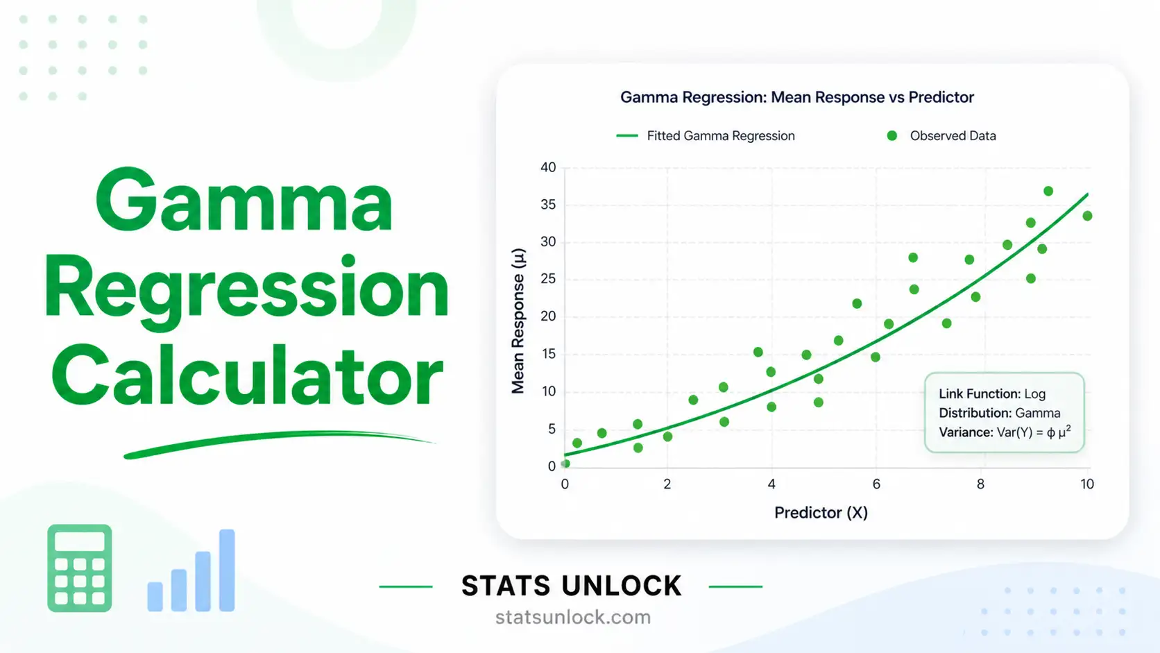
① Fitted vs Observed (Y > 0)
② Deviance Residuals vs Fitted
③ Q-Q Plot of Deviance Residuals
④ Outcome Histogram + Gamma Density
🧠 4. Plain-Language Interpretation
📖 Subsection 1 — Detailed Interpretation Results
📝 Subsection 2 — How to Write Your Results in Research (5 Examples)
Five copy-ready reporting templates for the gamma regression results — APA 7, dissertation, plain-language, conference abstract, and pre-registered open-science formats. Each updates automatically after you run the analysis.
🎯 5. Conclusion
Run the analysis to generate a detailed conclusion.
The conclusion section synthesises your gamma regression findings, model adequacy, practical implications, and limitations into a publication-ready closing statement.
🎯 6. When to Use Gamma Regression
This free gamma regression calculator is designed for analysing positive, right-skewed continuous outcomes — for example healthcare costs, insurance claim amounts, reaction times, rainfall, or hospital length of stay. Use it whenever a normal-errors linear regression would predict negative or implausible values for a strictly positive outcome.
✅ Use Gamma Regression When:
- Your outcome variable is strictly positive (Y > 0) and continuous.
- The distribution of Y is right-skewed (long upper tail).
- Variance increases with the mean (variance ∝ mean²).
- You want multiplicative interpretation of effects (with the log link).
- Linear regression of Y or log(Y) gives biased predictions or heteroscedastic residuals.
- Observations are independent (no nested/repeated structure).
📌 Real-World Examples
🌳 Decision Tree — Is Gamma Regression Right for My Data?
✅ 7. Assumption Checks
🧮 8. Technical Notes — Formulas & Derivations
Gamma GLM Specification
g(μ_i) = β₀ + β₁ X_i (linear predictor η_i)
Var(Y_i) = φ · μ_i²
Where:
• μ_i = expected value of Y for observation i
• φ = dispersion parameter (estimated from residuals)
• g(·) = link function (log, inverse, or identity)
• β₀, β₁ = intercept and slope coefficients on the link scale
Common Link Functions
Inverse link: g(μ) = 1/μ → μ = 1/η (canonical)
Identity link: g(μ) = μ → μ = η
The log link is most common because exp(η) is always positive, ensuring valid predictions.
Estimation — Iteratively Reweighted Least Squares (IRLS)
W = diag(1 / [Var(μ) · g'(μ)²])
z = η + (y − μ) · g'(μ)
Iterations continue until the deviance change drops below 1e-8. The Fisher information at convergence gives the standard errors for β.
Deviance & Goodness of Fit
Pearson χ² = Σ (y_i − μ_i)² / μ_i²
φ̂ = Pearson χ² / (n − p)
Residual deviance approximates a chi-square distribution with (n − p) degrees of freedom under correct model specification. Smaller deviance = better fit.
Pseudo R² (McFadden)
D_null = deviance of intercept-only model. Values 0.2–0.4 indicate excellent fit.
AIC (Akaike Information Criterion)
k = number of estimated parameters. Lower AIC = better model. Used to compare nested or non-nested gamma GLMs.
📘 9. How to Use This Gamma Regression Calculator
A complete walkthrough — using the built-in Healthcare Costs dataset as a worked example.
❓ 10. Frequently Asked Questions
Q1. What is gamma regression and when should I use it?
Gamma regression is a generalized linear model (GLM) for continuous, strictly positive, right-skewed outcomes such as healthcare costs, insurance claims, reaction times, or rainfall amounts. Use it when your outcome is always greater than zero and the variance grows with the mean — situations where ordinary linear regression would predict implausible negative values or violate the constant-variance assumption.
Q2. What is the difference between gamma regression and linear regression?
Linear regression assumes a normally distributed outcome with constant variance. Gamma regression assumes a gamma-distributed outcome with variance proportional to the mean squared, which is far more realistic for skewed positive data. Gamma regression also uses a non-identity link function (typically log), guaranteeing positive predictions.
Q3. What does the log link function do in gamma regression?
The log link sets log(μ) = β₀ + β₁X, so predicted means μ = exp(β₀ + β₁X) are always positive. Coefficients become multiplicative: exp(β₁) is the factor by which the mean changes per unit increase in X. The log link is the most common choice in practice.
Q4. How do I interpret gamma regression coefficients?
With the log link, exp(β) is a multiplicative effect on the mean: exp(β) = 1.05 means a 5% increase in expected outcome per unit X. With the inverse link, the effect is on the reciprocal scale and is harder to interpret directly. Always exponentiate log-link coefficients when reporting practical effects.
Q5. What is the dispersion parameter (φ) in gamma regression?
The dispersion parameter φ controls the shape of the gamma distribution. Smaller φ values mean tighter clustering of outcomes around the predicted mean. The estimate φ̂ = Pearson χ² / (n − p) is standard. Values much larger than 1 may indicate model mis-specification, while very small values suggest near-deterministic relationships.
Q6. What assumptions does gamma regression require?
Five core assumptions: (1) outcomes are strictly positive (Y > 0); (2) the conditional distribution of Y is gamma; (3) observations are independent; (4) the link function is correctly specified; and (5) variance is proportional to the mean squared. Violations of (1) or (5) are most damaging.
Q7. How do I check goodness of fit in gamma regression?
Look at residual deviance versus residual degrees of freedom (a ratio close to 1 suggests adequate fit), AIC for model comparison, McFadden's pseudo R², and diagnostic plots of deviance residuals against fitted values. A funnel-shaped residual plot signals lingering heteroscedasticity.
Q8. Can gamma regression handle zeros in the outcome?
No. The gamma distribution has support on (0, ∞), so exact zeros are invalid. For semi-continuous data with exact zeros, fit a Tweedie GLM (with 1 < p < 2) or a two-part hurdle model (logistic for zero-vs-positive, then gamma for positive values).
Q9. How is gamma regression reported in APA 7th edition format?
Report the model fit (residual deviance, df, AIC, dispersion), exponentiated coefficients with 95% confidence intervals, and exact p-values. Use italics for all statistical symbols. Section 4 of this tool gives a fully filled-in APA 7 example you can copy directly.
Q10. What if my gamma regression p-value is not significant?
A non-significant predictor means the data don't provide sufficient evidence of a non-zero effect at your chosen alpha level. Possible causes: small sample size, low effect size, mis-specified link function, omitted variables, or the outcome doesn't actually follow a gamma distribution. Inspect diagnostic plots before concluding "no effect".
📚 11. References
The following peer-reviewed sources support the methodology, formulas, and interpretation guidelines used in this gamma regression calculator — a generalized linear model with multiplicative interpretation and built-in p-value reporting for right-skewed positive outcomes.
- Nelder, J. A., & Wedderburn, R. W. M. (1972). Generalized linear models. Journal of the Royal Statistical Society: Series A, 135(3), 370–384. https://doi.org/10.2307/2344614
- McCullagh, P., & Nelder, J. A. (1989). Generalized Linear Models (2nd ed.). London: Chapman & Hall/CRC. https://doi.org/10.1201/9780203753736
- Hardin, J. W., & Hilbe, J. M. (2018). Generalized Linear Models and Extensions (4th ed.). College Station, TX: Stata Press.
- Dobson, A. J., & Barnett, A. G. (2018). An Introduction to Generalized Linear Models (4th ed.). Boca Raton, FL: CRC Press. https://doi.org/10.1201/9781315182780
- Manning, W. G., Basu, A., & Mullahy, J. (2005). Generalized modeling approaches to risk adjustment of skewed outcomes data. Journal of Health Economics, 24(3), 465–488. https://doi.org/10.1016/j.jhealeco.2004.09.011
- Manning, W. G., & Mullahy, J. (2001). Estimating log models: To transform or not to transform? Journal of Health Economics, 20(4), 461–494. https://doi.org/10.1016/S0167-6296(01)00086-8
- de Jong, P., & Heller, G. Z. (2008). Generalized Linear Models for Insurance Data. Cambridge University Press. https://doi.org/10.1017/CBO9780511755408
- Faraway, J. J. (2016). Extending the Linear Model with R (2nd ed.). Boca Raton, FL: Chapman & Hall/CRC. https://doi.org/10.1201/9781315382722
- Fox, J. (2016). Applied Regression Analysis and Generalized Linear Models (3rd ed.). Thousand Oaks, CA: Sage.
- Zuur, A. F., Ieno, E. N., Walker, N. J., Saveliev, A. A., & Smith, G. M. (2009). Mixed Effects Models and Extensions in Ecology with R. Springer. https://doi.org/10.1007/978-0-387-87458-6
- Wood, S. N. (2017). Generalized Additive Models: An Introduction with R (2nd ed.). CRC Press. https://doi.org/10.1201/9781315370279
- Akaike, H. (1974). A new look at the statistical model identification. IEEE Transactions on Automatic Control, 19(6), 716–723. https://doi.org/10.1109/TAC.1974.1100705
- R Core Team (2024). R: A language and environment for statistical computing. R Foundation for Statistical Computing. https://www.R-project.org/
- Pinheiro, J. C., & Bates, D. M. (2000). Mixed-Effects Models in S and S-PLUS. Springer. https://doi.org/10.1007/b98882
- American Psychological Association. (2020). Publication Manual of the American Psychological Association (7th ed.). https://doi.org/10.1037/0000165-000


