What is the intraclass correlation coefficient (ICC) in a mixed model?

The ICC is the share of the total variance that lies between clusters: ICC = between-cluster variance divided by total variance. It tells you how strongly observations within the same cluster resemble each other. An ICC near 0 means clustering barely matters; an ICC near 1 means cluster membership explains most of the variation.

How many clusters do I need for a mixed model?

As a rule of thumb you want at least 5 to 10 clusters to estimate a between-cluster variance, and 30 or more clusters for trustworthy standard errors on that variance. With very few clusters the ICC and variance components are estimated imprecisely, even if the total sample is large.

What is the difference between AIC and BIC here?

AIC and BIC are model-fit scores; lower is better. They let you compare the mixed model against a simpler model (such as one with no random effect). BIC penalises extra parameters more strongly than AIC, so it favours simpler models, especially with large samples.

Linear Mixed Model (LMM) Calculator – Free REML, ICC & Random Intercept Tool

Linear Mixed Model (LMM) Calculator – Free Online Random Intercept & ICC Tool

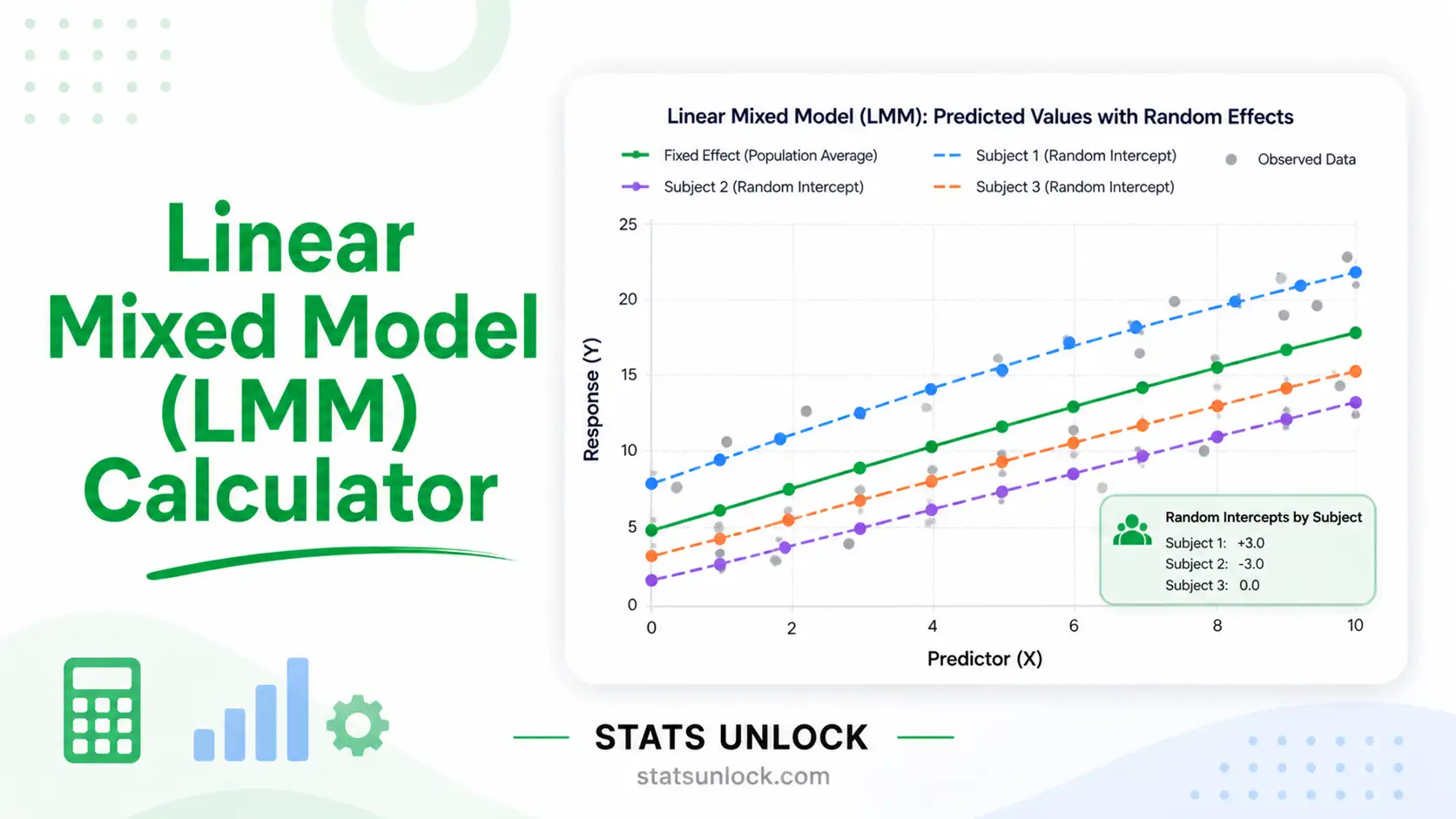
Linear Mixed Model (LMM) Calculator

Fit a random-intercept linear mixed model to clustered data — get REML variance components, the intraclass correlation (ICC), random intercepts (BLUPs), AIC/BIC, and publication-ready charts.

Mixed Effects Random Intercept Multilevel REML Free Online

📥 Enter Your Data

Load a sample dataset

Each cluster (subject, site, school, plot…) is one row. Enter the outcome values comma-separated. The cluster name is fully editable.

Upload CSV or Excel file:

Supports .csv, .txt, .xlsx, .xls — headers detected automatically. Click the columns that should each become a cluster — every selected column is loaded as a separate cluster.

Click any sample to load it instantly into the editable cluster rows on the first tab.

Significance level (α)

Estimation method

Outcome variable name

📊 Results

Model Summary

Random Effects — Cluster Intercepts (BLUPs)

📈 Visualizations

1. Outcome by Cluster (box + points)

2. Cluster Means ± SE vs Grand Mean

3. Variance Decomposition (ICC)

4. Shrinkage: Raw Mean → BLUP

⬇️ Export Your Results

🔗 Copy summary to clipboard

✅ Assumption Checks

🧠 Interpretation of Results

✍️ How to Write Your Results in Research

🏁 Conclusion

📐 Technical Notes & Formulas

A. Formulas Used

The random-intercept linear mixed model for observation i in cluster j:

y_ij = β0 + u_j + e_ij

Where:
  y_ij  = outcome value i within cluster j
  β0    = fixed (overall) intercept — the grand mean level
  u_j   = random intercept for cluster j,   u_j ~ N(0, σ²_u)
  e_ij  = residual error,                   e_ij ~ N(0, σ²_e)
  σ²_u  = between-cluster variance
  σ²_e  = within-cluster (residual) variance

Intraclass correlation coefficient (ICC):

ICC = σ²_u / (σ²_u + σ²_e)

  = proportion of total variance that lies BETWEEN clusters
  range 0 → 1 ; higher means stronger clustering

Variance components by REML / ANOVA decomposition:

SSB = Σ n_j (ȳ_j − ȳ)²          (between, df = k−1)
SSW = Σ Σ (y_ij − ȳ_j)²         (within,  df = N−k)
MSB = SSB / (k−1)   ;   MSW = SSW / (N−k)
F   = MSB / MSW       (tests H0: σ²_u = 0)

ANOVA estimator:
  σ̂²_e = MSW
  σ̂²_u = (MSB − MSW) / n0 ,   n0 = (N − Σn_j²/N)/(k−1)

REML refines σ̂²_u, σ̂²_e by maximising the restricted likelihood
of the compound-symmetry marginal model V_j = σ²_e·I + σ²_u·J.

Where:
  k     = number of clusters
  N     = total number of observations
  n_j   = number of observations in cluster j
  ȳ_j   = mean of cluster j
  ȳ     = grand (overall) mean

Best Linear Unbiased Predictors (random intercepts), with shrinkage:

û_j = λ_j (ȳ_j − β0) ,   λ_j = σ²_u / (σ²_u + σ²_e / n_j)
BLUP_j = β0 + û_j

  λ_j  = shrinkage factor (smaller clusters shrink more toward β0)

Model fit:

AIC = −2·logL + 2p        BIC = −2·logL + p·ln(N)     (p = 3 params)
LRT = 2(logL_full − logL_null)   vs  ½·χ²(0) + ½·χ²(1)  boundary mixture

B. Technical Notes

This tool fits the random-intercept-only mixed model (one-way variance-components model). It is the foundational LMM and the correct model when each cluster supplies repeated measurements of a single outcome.
REML is used by default and reproduces the variance components reported by lme4::lmer(y ~ 1 + (1|cluster)) in R and MixedLM in Python statsmodels.
The F-test is exact under normality and tests whether the between-cluster variance is zero. The likelihood-ratio test uses a 50:50 boundary correction because a variance cannot be negative.
For models with predictors (random slopes, crossed/nested effects, non-normal outcomes), fit the model in dedicated software — this calculator covers the intercept-only case.

🎯 When to Use a Linear Mixed Model

This free linear mixed model tool is designed for data that are grouped, nested, or repeated. A mixed model adds a random intercept so that correlated observations inside the same cluster are modelled correctly, instead of being wrongly treated as independent.

Decision Checklist

✅ Your observations fall into natural clusters (subjects, sites, schools, litters, plots, hospitals).
✅ Observations within a cluster are likely to be more similar to each other than to observations in other clusters.
✅ Your outcome is continuous (interval or ratio scale).
✅ You want to separate within-cluster variation from between-cluster variation (and get the ICC).
❌ Do NOT use if every observation is independent with no grouping → use ordinary regression or a t-test/ANOVA.
❌ Do NOT use this intercept-only version if you need predictor slopes → fit a full mixed model with fixed covariates.
❌ Do NOT use if the outcome is binary or a count → use a generalized linear mixed model (GLMM).

Real-World Examples

Ecology / wildlife: Repeated body-mass measurements of animals at several camera-trap sites — sites are clusters; ICC shows how much mass varies between sites.
Education: Test scores of students nested in classrooms — classrooms are clusters.
Medicine: Blood-pressure readings taken several times per patient — patients are clusters.
Agriculture: Yield from several plants within each field plot — plots are clusters.

Sample Size Guidance

At least 5–10 clusters to estimate a between-cluster variance at all.
30+ clusters for a trustworthy standard error on the variance component and the ICC.
A few observations per cluster is fine; balance across clusters is helpful but not required.

Related Models — Decision Tree

Grouped / nested data? ├─ Continuous outcome, random intercept only → THIS TOOL (LMM, random intercept) ├─ Continuous outcome + predictor slopes vary → Random-slopes LMM ├─ Binary / count outcome → GLMM (mixed logistic / mixed Poisson) └─ No grouping → OLS regression / ANOVA / t-test

📖 How to Use This Linear Mixed Model Calculator

Enter your data. On the “Type / Paste Data” tab, put each cluster on its own row and type the outcome values comma-separated, e.g. 52, 48, 55, 61, 47. Rename clusters freely. Example: four study sites with several measurements each.
Or load a sample. Pick from the dropdown (or the Quick Sample tab) to load a ready dataset such as “Camera-Trap Sites”.
Or upload a file. On the Upload tab, choose a CSV/Excel file and click each column that should become a cluster; selected columns load as separate clusters.
Configure settings. Choose α (default 0.05), the estimation method (REML recommended), and the outcome name shown in your report.
Run the analysis. Click “Run Linear Mixed Model”. Nothing is computed until you click.
Read the summary cards. They show the ICC, between- and within-cluster variance, and the random-effect p-value (green = significant).
Read the model table. It lists the fixed intercept with its standard error, both variance components, the ICC, AIC/BIC, and the F / likelihood-ratio tests.
Read the random effects table. Each cluster’s raw mean, shrinkage factor, predicted intercept (BLUP), and deviation from the overall mean.
Study the four charts. Distribution by cluster, cluster means vs grand mean, the variance split (ICC), and the shrinkage of raw means toward the BLUPs.
Export. Use Download Doc for a text report or Download PDF for a print-ready version; copy any APA / thesis / plain-language template from the interpretation section.

❓ Frequently Asked Questions

Q1. What is a linear mixed model (LMM) and when should I use it?

A linear mixed model is a regression that combines fixed effects with random effects. The random-intercept model here is for data grouped into clusters — subjects, sites, schools, plots. Use it when observations within a cluster are correlated and ordinary regression would treat them, incorrectly, as independent.

Q2. What is the intraclass correlation coefficient (ICC)?

The ICC is the proportion of total variance that lies between clusters: between-cluster variance divided by total variance. An ICC near 0 means clustering hardly matters; near 1 means cluster membership explains most of the variation. It is also the expected correlation between two observations from the same cluster.

Q3. What does REML mean and why use it?

REML is Restricted Maximum Likelihood. It estimates the variance components after removing the fixed effects, which corrects the downward bias that ordinary maximum likelihood has for variances in small samples. This tool uses REML, so its values match R’s lme4 and Python’s statsmodels.

Q4. What is a random intercept and what are BLUPs?

A random intercept gives each cluster its own baseline level around the overall mean. BLUPs (Best Linear Unbiased Predictors) are the predicted cluster intercepts. They are shrunk toward the overall mean — small clusters shrink more — which makes them more stable than raw cluster means.

Q5. How do I interpret the p-value for the random effect?

The F-test and likelihood-ratio test ask whether the between-cluster variance is zero. A small p-value (say below your α) means clusters differ significantly and the mixed model is justified. Because a variance cannot be negative, the likelihood-ratio test halves the naive p-value as a boundary correction.

Q6. What assumptions does a linear mixed model make?

Residuals should be roughly normal with constant variance; the random cluster effects should be roughly normal; clusters should be independent; and the model should be correctly specified. Check the residual spread, a Q-Q plot of residuals, and a Q-Q plot of the cluster effects.

Q7. How many clusters do I need?

At least 5–10 clusters to estimate a between-cluster variance, and 30 or more for a reliable standard error on that variance and the ICC. With very few clusters the variance components are imprecise even when the total sample is large.

Q8. What is the difference between AIC and BIC?

Both are model-fit scores where lower is better, used to compare competing models. BIC penalises extra parameters more strongly than AIC, so it tends to favour simpler models, especially as the sample grows.

Q9. Can I use this calculator for my thesis or published research?

Yes for learning, checking, and exploratory work. For a formal thesis or publication, reproduce the result in peer-reviewed software (R lme4, Python statsmodels, SPSS, SAS) and cite it. You may cite this tool as: STATS UNLOCK. (2025). Linear mixed model calculator. https://statsunlock.com.

Q10. What if my F-test is not significant?

A non-significant result means the data do not provide clear evidence that clusters differ in their baseline level — it does not prove they are identical. With few clusters or small samples the test may simply lack power. Always read the ICC and the size of the between-cluster variance alongside the p-value.

📚 References

The following references support the statistical methods used in this linear mixed model calculator, covering variance components estimation, intraclass correlation, and best practices in multilevel / mixed-effects modelling.

Laird, N. M., & Ware, J. H. (1982). Random-effects models for longitudinal data. Biometrics, 38(4), 963–974. https://doi.org/10.2307/2529876
Harville, D. A. (1977). Maximum likelihood approaches to variance component estimation and to related problems. Journal of the American Statistical Association, 72(358), 320–338. https://doi.org/10.1080/01621459.1977.10480998
Patterson, H. D., & Thompson, R. (1971). Recovery of inter-block information when block sizes are unequal. Biometrika, 58(3), 545–554. https://doi.org/10.1093/biomet/58.3.545
Henderson, C. R. (1975). Best linear unbiased estimation and prediction under a selection model. Biometrics, 31(2), 423–447. https://doi.org/10.2307/2529430
Bates, D., Mächler, M., Bolker, B., & Walker, S. (2015). Fitting linear mixed-effects models using lme4. Journal of Statistical Software, 67(1), 1–48. https://doi.org/10.18637/jss.v067.i01
Raudenbush, S. W., & Bryk, A. S. (2002). Hierarchical linear models: Applications and data analysis methods (2nd ed.). SAGE Publications.
Snijders, T. A. B., & Bosker, R. J. (2012). Multilevel analysis: An introduction to basic and advanced multilevel modeling (2nd ed.). SAGE Publications.
Gelman, A., & Hill, J. (2007). Data analysis using regression and multilevel/hierarchical models. Cambridge University Press. https://doi.org/10.1017/CBO9780511790942
Nakagawa, S., & Schielzeth, H. (2010). Repeatability for Gaussian and non-Gaussian data: A practical guide for biologists. Biological Reviews, 85(4), 935–956. https://doi.org/10.1111/j.1469-185X.2010.00141.x
Self, S. G., & Liang, K.-Y. (1987). Asymptotic properties of maximum likelihood estimators and likelihood ratio tests under nonstandard conditions. Journal of the American Statistical Association, 82(398), 605–610. https://doi.org/10.1080/01621459.1987.10478472
Searle, S. R., Casella, G., & McCulloch, C. E. (1992). Variance components. John Wiley & Sons. https://doi.org/10.1002/9780470316856
Seabold, S., & Perktold, J. (2010). statsmodels: Econometric and statistical modeling with Python. Proceedings of the 9th Python in Science Conference, 92–96. https://doi.org/10.25080/Majora-92bf1922-011
Pinheiro, J. C., & Bates, D. M. (2000). Mixed-effects models in S and S-PLUS. Springer. https://doi.org/10.1007/b98882
Bolker, B. M., Brooks, M. E., Clark, C. J., Geange, S. W., Poulsen, J. R., Stevens, M. H. H., & White, J.-S. S. (2009). Generalized linear mixed models: A practical guide for ecology and evolution. Trends in Ecology & Evolution, 24(3), 127–135. https://doi.org/10.1016/j.tree.2008.10.008
American Psychological Association. (2020). Publication manual of the American Psychological Association (7th ed.). APA. https://doi.org/10.1037/0000165-000