
Genotype Calculator
Enter two parent genotypes and get every offspring genotype and phenotype, the full Punnett square, the genotypic and phenotypic ratios, and a chi-square test on your real counts. Genotype vs phenotype, homozygous and heterozygous, all explained in plain English.
⚡ 0. Quick Answer
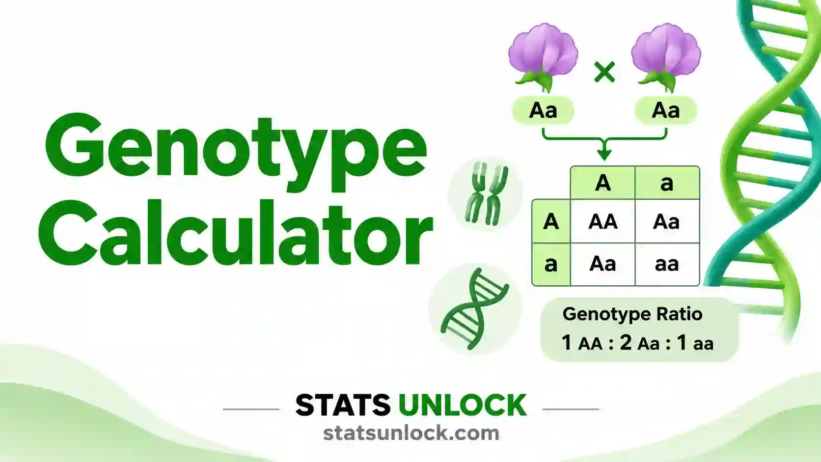
A genotype is the pair of alleles an organism carries for a gene, written as AA, Aa or aa. Crossing Aa × Aa gives genotypes in a 1 AA : 2 Aa : 1 aa ratio and phenotypes in a 3 : 1 ratio.
The genotype is the genetic instruction. The phenotype is what that instruction produces in a real body and a real environment. Two genotypes, AA and Aa, can give the same phenotype when one allele is dominant, which is why you cannot always read a genotype from the outside.
Rule of thumb: a dihybrid cross AaBb × AaBb gives 9:3:3:1. If your counts give a chi-square p-value of 0.05 or more (below 7.815 on 3 df), they fit Mendel’s ratio.
Key takeaways
- A genotype is the allele pair for a gene: AA homozygous dominant, Aa heterozygous, aa homozygous recessive.
- The difference between genotype and phenotype: AA and Aa both show the dominant phenotype, so a 1:2:1 genotypic ratio becomes a 3:1 phenotypic ratio.
- A parent with h heterozygous genes makes 2h gametes, so AaBb makes 4 and a dihybrid Punnett square has 16 squares.
- Mendel’s 556 dihybrid pea seeds give χ² = 0.470, p = 0.925: a near-perfect fit to 9:3:3:1.
- A p-value below 0.05 means the data do not fit; in a two-gene cross the usual cause is linkage.
📚 1. What Is a Genotype?
Genotype definition in biology: a genotype is the set of alleles an organism carries at one or more genes. An allele is one version of a gene. Because most animals and plants are diploid, they carry two alleles for each gene, one from each parent. We write them as two letters: a capital letter for the dominant allele and a small letter for the recessive allele.
The word was coined by the Danish botanist Wilhelm Johannsen in 1909 and explained in English in 1911, together with its partner word, phenotype. Johannsen wanted to separate what an organism carries from what it shows. That split is still the heart of genetics.
What is the difference between genotype and phenotype? The genotype is the genetic code, such as Aa. The phenotype is the observable result, such as purple flowers, blood group A, or a disease. Phenotype depends on the genotype and on the environment. A plant with tall genotype grown in poor soil can still be short.
A worked one-liner: in peas, R (round seed) is dominant over r (wrinkled). Crossing two Rr plants gives 1/4 RR, 2/4 Rr and 1/4 rr. RR and Rr both look round, so 3/4 of seeds are round and 1/4 wrinkled. Mendel counted 5,474 round and 1,850 wrinkled seeds, a ratio of 2.96 to 1.
Types of genotype. For one gene with two alleles there are three genotypes. Homozygous dominant (AA) carries two dominant alleles. Heterozygous (Aa) carries one of each, so it is made of two different alleles. Homozygous recessive (aa) carries two recessive alleles, so it is made of the same allele twice. Only aa shows the recessive phenotype under complete dominance.
Who uses genotypes: plant and animal breeders predict which crosses give the trait they want. Genetic counsellors give couples the risk of a recessive disease. Clinical labs use SNP genotyping to choose drug doses. Ecologists and wildlife researchers genotype hair, scat or tissue samples to identify individuals and measure genetic diversity.
Genotype vs phenotype vs allele vs haplotype
| Term | What it is | Example | Can you see it? |
|---|---|---|---|
| Allele | One version of a gene | R or r | No |
| Genotype | The pair (or set) of alleles an organism carries | Rr | Not directly; it needs a cross or a DNA test |
| Phenotype | The observable trait the genotype produces | Round seed | Yes |
| Haplotype | The set of alleles on one chromosome, inherited together | R-Y on one chromosome, r-y on the other | No, it needs phasing |
| Genotyping | A lab test that reads the genotype from DNA | A SNP array calls a cow as GG, Gg or gg | Gives the genotype directly |
🧮 2. Set Up Your Data
Genes, dominance and trait names
Every trait name is editable and flows into the Punnett square, the tables, the charts and the report.
Upload a file with one offspring genotype per row, for example the output of a SNP genotyping run or a scoring sheet (Aa, AA, aa...). The tool tallies each genotype class and fills the observed counts for you. Set the parents on the first tab first.
One row per class, in the order the cross produces them. Empty cells count as 0.
📊 3. Results
🧠 4. Interpretation of Results, In Detail
4.1 What a genotype result actually tells you
Each genotype in the table is a probability for one offspring. If P(aa) = 25%, each child, seed or chick has a one in four chance of being aa. It does not mean that exactly one in every four offspring will be aa. In a litter of four puppies, all four can be aa, and that happens with probability (1/4)4 = 0.39%.
4.2 Genotypic ratio vs phenotypic ratio
The genotypic ratio counts distinct allele combinations. The phenotypic ratio counts distinct visible traits. Under complete dominance the phenotypic ratio is shorter, because AA and Aa collapse into one class: 1:2:1 becomes 3:1, and the dihybrid 1:2:1:2:4:2:1:2:1 becomes 9:3:3:1. Under incomplete dominance or codominance the heterozygote has its own phenotype, so the two ratios are the same.
4.3 Homozygous and heterozygous genotypes in the output
The zygosity column labels every gene. A homozygous genotype has two copies of the same allele (AA or aa) and always breeds true for that gene. A heterozygous genotype has two different alleles (Aa) and passes each one to half its gametes. Chart 4 shows the share of each zygosity class per gene. For any Aa × Aa gene it is 25% / 50% / 25%.
4.4 Reading the chi-square result
The chi-square test asks one question: are the gaps between observed and expected counts small enough to be chance? A p-value of 0.05 or more says yes, so the data fit the ratio. A p-value below 0.05 says the gaps are larger than chance usually gives. A good fit does not prove the model. It means your data give no reason to reject it.
4.5 Why p is not the probability that Mendel was right
p = 0.925 does not mean a 92.5% chance that the 9:3:3:1 model is true. It means that if the model is true, about 92.5% of experiments of this size would show deviations at least this large. Very high p-values across many experiments can even be suspicious, which is exactly the point Fisher raised in 1936 about Mendel’s own data.
4.6 What a failed fit usually means
In a two-gene cross the most common cause is linkage: the genes sit near each other on one chromosome, so parental combinations appear too often and recombinant ones too rarely. Other causes are a lethal genotype (for example a 2:1 ratio instead of 3:1), epistasis (9:3:4 or 9:7 instead of 9:3:3:1), mis-scored phenotypes, or a parent whose genotype was wrong.
4.7 Expected counts below 5
The chi-square p-value is an approximation that works when every expected count is 5 or more. Below that, it can be badly off. The calculator flags these classes. Count more offspring, merge rare classes, or use an exact binomial test, which for a two-class cross is easy to run in R or Python (Section 10.5 and 11.5).
4.8 Genotype vs phenotype in the real world
A Punnett square assumes the phenotype follows from the genotype alone. Real traits are messier. Penetrance below 100% means some carriers never show the trait. Variable expressivity means the trait shows at different strengths. Most human traits, such as height, are polygenic and depend on hundreds of genes plus the environment, so one Punnett square cannot predict them.
4.9 Allele frequencies from genotyped offspring
When you enter counts per genotype, the tool also gives the allele frequency p = (2 × AA + Aa) ÷ (2 × n). For an Aa × Aa cross the expected value is 0.5. A big gap can point to unequal gamete success, called segregation distortion, or to a genotyping error such as allele dropout that turns real heterozygotes into homozygotes.
4.10 Practical judgement
Start with the expected ratio. Then look at the observed vs expected chart before the p-value: it shows which class is off. If one class is short in every replicate, suspect lower survival of that genotype. If the two parental classes are both high, suspect linkage. Only then report the chi-square value, with n and df.
✍ 5. How to Report Your Genotype Results
📌 Key conventions for this style
- Name the parents, the cross type and the assumption of independent assortment.
- Report χ², df, p and n together.
- Name how genotypes or phenotypes were scored: by eye, PCR-RFLP, TaqMan, or a SNP array, with the kit or instrument.
- Italicise gene symbols in the final manuscript.
📌 Key conventions for this style
- Explain why that ratio is expected before you test it.
- Show the Punnett square as a figure.
- Discuss what a failed fit would mean: linkage, lethality or epistasis.
- Name the software and version used.
📌 Key conventions for this style
- Record the parent IDs, the date the cross was set and the date it was scored.
- Write who scored the offspring and whether they were blind to the expected ratio.
- Note dead or unscorable offspring, since they can bias the ratio.
- Keep the raw tally sheet.
📌 Key conventions for this style
- One sentence for the ratio, one for the test, one for the meaning.
- Use the APA style χ²(df) = value, p = value.
- Put the observed vs expected bar chart on the poster.
- Avoid symbols a general audience will not know.
📌 Key conventions for this style
- List every genotype class, even those with zero offspring.
- Give raw counts, not only percentages.
- Deposit SNP genotype calls in a public archive where the journal requires it.
- State the genotyping call rate and error rate.
∑ 6. Formulas Used
🔀 7. Genotype Calculation Flowchart, Step by Step
This flowchart shows how the genotype and phenotype ratios of a cross are calculated, step by step, from two parent genotypes to a chi-square verdict. Every box uses the same worked example as the Excel, R and Python sections: Mendel’s dihybrid pea cross RrYy × RrYy, with 556 F2 seeds counted.
Check any box yourself: the Excel sheet in Section 9, the R script in Section 10 and the Python script in Section 11 all return χ² = 0.4700 and p = 0.9254 for these counts.
📝 8. How to Use This Genotype Calculator
- Enter Parent 1's genotype. Type one letter per gene, two letters per gene, capital for the dominant allele, for example RrYy. Up to 4 genes are supported.
- Enter Parent 2's genotype. Use the same genes in the same order, for example RrYy or rryy for a test cross.
- Set the dominance for each gene. Choose complete dominance, incomplete dominance or codominance. This decides whether the heterozygote has its own phenotype.
- Name the traits. Edit the dominant, recessive and heterozygote trait names, such as Round and Wrinkled. They flow into the Punnett square, tables, charts and report.
- Choose a sample dataset if you want to explore. Ten built-in crosses cover Mendel's peas, a test cross, incomplete dominance, codominance, a carrier couple, SNP genotyping and a failed fit caused by linked genes.
- Add observed counts. Type offspring counts per phenotype or genotype class, comma separated, in the order shown under the box. Or set observed counts to None for expected ratios only.
- Or upload genotype calls. On the Upload tab, choose a CSV or Excel file with one offspring genotype per row. The tool tallies each class and fills the counts for you.
- Ask for one genotype's probability. Type a target genotype such as rryy to get its probability as a fraction and a percentage.
- Press Calculate Genotypes. Nothing is computed until you press the button. Changing any input clears the old results so you never read stale numbers.
- Read, copy and download the results. Check the Punnett square, the genotype and phenotype tables, the chi-square verdict and the four charts. Section 5 fills five report styles, and the buttons save a text report or a PDF.
📈 9. How to Calculate Genotype Ratios in Excel
Excel has no Punnett square function, but everything you need is basic arithmetic: expected counts, the chi-square sum and one p-value function. The easy part is the ratio. The parts that trip people up are absolute references when you fill a formula down, and Excel turning gene names into dates.
=CHISQ.TEST(B2:B5,D2:D5) and press Enter. For Mendel’s dihybrid peas it returns 0.9254.9.1 The functions you need
| You want | Excel function | Note |
|---|---|---|
| Total offspring | =SUM(B2:B5) | Use raw counts, never percentages |
| Expected count | =$B$6*C2/$C$6 | Dollar signs lock the totals when you fill down |
| Chi-square contribution | =(B2-D2)^2/D2 | One per class, then sum them |
| p-value from χ² | =CHISQ.DIST.RT(E6,3) | Second argument is df = classes − 1 |
| p-value in one step | =CHISQ.TEST(B2:B5,D2:D5) | Uses df = rows − 1 automatically |
| Critical value | =CHISQ.INV.RT(0.05,3) | Returns 7.815 |
| Genotype in a Punnett square | =IF(EXACT($A2,UPPER($A2)),$A2&B$1,B$1&$A2) | If the row allele is a capital, it goes first |
| Count one genotype | =COUNTIF(B2:C3,"Rr") | COUNTIF is not case sensitive, see 9.3 |
| Reduce a ratio | =B2/GCD($B$2:$B$5) | Turns 9, 3, 3, 1 squares into the 9:3:3:1 ratio |
9.2 Step by step
1 Type the phenotype classes and observed counts
Put each phenotype class in column A and its observed count in column B. Add a Total row with =SUM.
=SUM(B2:B5)Mendel’s four classes: 315, 108, 101 and 32, which sum to 556 seeds in B6.
2 Add the expected ratio parts
In column C type the ratio from the cross: 9, 3, 3, 1. The total in C6 is 16, the number of Punnett squares.
=SUM(C2:C5)The ratio parts 9, 3, 3 and 1 sum to 16 in C6.
3 Calculate expected counts with locked totals
In D2 multiply the total offspring by the class share, then fill down. The dollar signs keep B6 and C6 fixed.
=$B$6*C2/$C$6D2 returns 312.75; filled down it gives 104.25, 104.25 and 34.75.
4 Add the chi-square contributions
In E2 compute (O − E)² ÷ E and fill down. Sum the column in E6.
=(B2-D2)^2/D2 =SUM(E2:E5)Contributions of 0.0162, 0.1349, 0.1013 and 0.2176 give χ² = 0.4700 in E6.
5 Turn χ² into a p-value
Use the right-tail chi-square function with df = 3. Add the critical value beside it so the verdict is obvious.
=CHISQ.DIST.RT(E6,3) =IF(B8>=0.05,"Fits","Does not fit")p = 0.9254 in B8, far above 0.05, so the counts fit 9:3:3:1.
6 Build a Punnett square with a formula
Type the gametes of one parent down column A and the other across row 1. One formula, filled across and down, writes every genotype with the capital letter first.
=IF(EXACT($A2,UPPER($A2)),$A2&B$1,B$1&$A2)Rr × Rr gives RR, Rr, Rr and rr: the 1:2:1 genotypic ratio.
9.3 The awkward cases
Dihybrid Punnett squares. For two genes, join the gene-by-gene results: =IF(EXACT(LEFT($A2),UPPER(LEFT($A2))),LEFT($A2)&LEFT(B$1),LEFT(B$1)&LEFT($A2))&IF(EXACT(RIGHT($A2),UPPER(RIGHT($A2))),RIGHT($A2)&RIGHT(B$1),RIGHT(B$1)&RIGHT($A2)). The classic mistake is forgetting that a gamete like Ry has one letter per gene, so LEFT and RIGHT pick the right allele.
Counting genotypes. COUNTIF ignores case, so it counts Rr, RR and rr as the same text. Use =SUMPRODUCT(--EXACT(B2:E5,"Rr")) instead. This is the most common silent error in student spreadsheets.
Percentages instead of counts. Chi-square must use raw counts. Feeding it 56.7%, 19.4% and so on gives a statistic that depends on how you scaled the numbers, not on your sample size.
9.4 Why your Excel answer might differ from R or Python
| Situation | What happens | Fix |
|---|---|---|
| Blank cells in the observed range | CHISQ.TEST skips the pair, so df shrinks | Type 0 for a class with no offspring |
| Counts stored as text | SUM ignores them, so n is too small | Look for green triangles, then Convert to Number |
| Expected given as proportions | CHISQ.TEST compares counts with proportions and returns p near 0 | Multiply proportions by n first |
| Yates correction | R’s chisq.test on a 2 × 2 table corrects by default; Excel never does | For goodness of fit, R does not correct, so all three agree |
| Rounded expected counts | Typing 313 instead of 312.75 shifts χ² in the third decimal | Keep the formula, not a typed value |
| Wrong df | CHISQ.DIST.RT with df 4 instead of 3 gives p = 0.976 | df is the number of classes minus 1 |
With the same counts, Excel, R and Python all give χ² = 0.4700 and p = 0.9254. Rounding shown on screen is not rounding stored: widen the column or use more decimals before you compare.
9.5 Charting observed vs expected in Excel
- Select the class names in A1:A5, then hold Ctrl and select B1:B5 and D1:D5.
- Choose Insert → Clustered Column.
- Colour observed and expected differently and add data labels so readers see the gaps.
- Put χ², df and p in the chart title, for example χ²(3) = 0.47, p = 0.93.
- For a Punnett square figure, use Home → Conditional Formatting → Text that Contains to colour each phenotype.
9.6 Excel errors you will probably hit
| Excel shows | Why | Fix |
|---|---|---|
#DIV/0! | An expected count is 0, often because the ratio part is blank | Remove classes the cross cannot produce |
#N/A from CHISQ.TEST | The observed and expected ranges are different sizes | Make both ranges the same number of rows |
#NUM! from CHISQ.DIST.RT | df is 0 or negative, or χ² is negative | Check df = classes − 1 and the contribution formula |
#VALUE! | Text such as "32 seeds" in a count cell | Keep only numbers in count columns |
| Gene name became a date | Autoformat of names such as SEPT2 | Format the column as Text before pasting |
| Punnett cell shows rR | Formula concatenates without sorting | Use the EXACT and UPPER test from 9.1 |
📈 10. How to Calculate Genotype Ratios in R
In R the one-liner is chisq.test(obs, p = c(9, 3, 3, 1) / 16), but that skips the part people get wrong: building the Punnett square and the ratio from the parent genotypes. The script below does the whole job in base R. It builds the gametes and the Punnett square, counts genotypes and phenotypes, tests the counts, prints a plain-English verdict and saves one 300 dpi figure.
Rscript. Change only the p1, p2, traits and obs lines to use your own cross.10.1 The complete script
R, base only, saves genotype_plot.png
# ============================================================
# Genotype calculator: Punnett square, genotype and phenotype
# ratios, and a chi-square goodness-of-fit test
# StatsUnlock - https://statsunlock.com/genotype-calculator/
# Base R only. No packages to install.
# ============================================================

# ---- 1. Your cross ------------------------------------------
# Parent genotypes: one letter per gene, capital = dominant allele
p1 <- "RrYy"
p2 <- "RrYy"

# Trait names for each gene: dominant first, then recessive
traits <- list(R = c("Round", "Wrinkled"),
               Y = c("Yellow", "Green"))

# Observed offspring per phenotype class, in the order printed below.
# Or read them from a file:
#   obs <- read.csv("counts.csv")$count
#   obs <- obs[!is.na(obs)]
obs <- c(315, 108, 101, 32)          # Mendel (1866), 556 F2 seeds

# ---- 2. Split each parent into genes ------------------------
split_genes <- function(g) {
  a <- strsplit(g, "")[[1]]
  sapply(seq(1, length(a), 2), function(i) paste(a[i], a[i + 1], sep = ""))
}
g1 <- split_genes(p1)
g2 <- split_genes(p2)
k  <- length(g1)

# Put the capital (dominant) allele first: "rR" becomes "Rr"
norm_pair <- function(x) {
  s <- strsplit(x, "")[[1]]
  paste(s[order(s != toupper(s))], collapse = "")
}

# ---- 3. Gametes: one allele from every gene -----------------
gametes <- function(genes) {
  opts <- lapply(genes, function(x) unique(strsplit(x, "")[[1]]))
  apply(expand.grid(rev(opts), stringsAsFactors = FALSE), 1,
        function(r) paste(rev(r), collapse = ""))
}
gam1 <- gametes(g1)
gam2 <- gametes(g2)

# ---- 4. Punnett square --------------------------------------
offspring <- function(a, b) {
  pa <- strsplit(a, "")[[1]]; pb <- strsplit(b, "")[[1]]
  paste(sapply(seq_len(k), function(i) norm_pair(paste0(pa[i], pb[i]))),
        collapse = "")
}
grid <- outer(gam1, gam2, Vectorize(offspring))
dimnames(grid) <- list(gam1, gam2)
cat("Punnett square:\n"); print(noquote(grid))

# ---- 5. Genotype and phenotype probabilities ----------------
geno_tab <- table(grid)
geno_p   <- geno_tab / sum(geno_tab)

phenotype <- function(gt) {
  s <- substring(gt, seq(1, 2 * k, 2), seq(2, 2 * k, 2))
  paste(sapply(seq_len(k), function(i) {
    dom <- any(strsplit(s[i], "")[[1]] == toupper(substr(s[i], 1, 1)))
    traits[[i]][ifelse(dom, 1, 2)]
  }), collapse = ", ")
}
phen <- table(sapply(grid, phenotype))
# order classes dominant-first, gene by gene
lvl <- apply(expand.grid(rev(traits))[, k:1, drop = FALSE], 1, paste, collapse = ", ")
phen <- phen[intersect(lvl, names(phen))]
phen_p <- phen / sum(phen)

ratio <- function(x) { g <- Reduce(function(a, b) if (b == 0) a else Recall(b, a %% b), x)
                       paste(x / g, collapse = ":") }
cat("\nGenotypic ratio :", ratio(as.vector(geno_tab)), "\n")
cat("Phenotypic ratio:", ratio(as.vector(phen)), "\n")
print(round(phen_p, 4))

# ---- 6. Chi-square goodness of fit --------------------------
expected <- sum(obs) * as.vector(phen_p)
test <- chisq.test(obs, p = as.vector(phen_p))
crit <- qchisq(0.95, df = length(obs) - 1)
cat(sprintf("\nn = %d, chi-square = %.4f, df = %d, critical = %.3f, p = %.4f\n",
            sum(obs), test$statistic, test$parameter, crit, test$p.value))
cat("Expected:", round(expected, 2), "\n")
cat(if (test$p.value >= 0.05) {
  "Verdict: the counts FIT the expected ratio (p >= 0.05).\n"
} else {
  "Verdict: the counts do NOT fit the expected ratio (p < 0.05).\n"
})

# ---- 7. One figure, 300 dpi ---------------------------------
set.seed(1)                          # nothing random here, kept for habit
cols <- c("#16a34a", "#2563eb", "#d97706", "#9333ea",
          "#0d9488", "#c2410c", "#0891b2", "#475569")[seq_along(obs)]
png("genotype_plot.png", width = 2700, height = 1800, res = 300)
par(mar = c(6.5, 5, 4, 1))
bp <- barplot(rbind(obs, expected), beside = TRUE,
              col = c("#2563eb", "#fbbf24"), border = NA,
              names.arg = names(phen), las = 2, cex.names = 0.8,
              ylab = "Offspring (count)", ylim = c(0, max(obs, expected) * 1.15))
legend("topright", c("Observed", "Expected"), fill = c("#2563eb", "#fbbf24"),
       border = NA, bty = "n")
title(main = sprintf("%s x %s: phenotypic ratio %s", p1, p2, ratio(as.vector(phen))),
      adj = 0, line = 2.2)
title(main = sprintf("chi-square = %.3f, df = %d, p = %.4f",
                     test$statistic, test$parameter, test$p.value),
      adj = 0, line = 0.8, font.main = 1, cex.main = 0.95)
invisible(dev.off())
cat("Saved genotype_plot.png\n")
Run it with Rscript genotype.R from a terminal, or paste it into the RStudio console. It prints the Punnett square, the 1:2:1:2:4:2:1:2:1 and 9:3:3:1 ratios, χ² = 0.4700, df = 3, p = 0.9254, and saves genotype_plot.png in your working directory (check it with getwd()).
10.2 What each part does
| Line or function | What it does, and why it is there |
|---|---|
| p1, p2 | The parent genotypes as plain text. One letter per gene, capital for the dominant allele. |
| traits | A named list of trait names, dominant first. The names become the phenotype classes. |
| obs | Observed counts in the same order as the printed phenotype classes. read.csv plus obs[!is.na(obs)] loads them from a file and drops blanks. |
| split_genes() | Cuts "RrYy" into "Rr" and "Yy" so each gene is handled on its own. |
| norm_pair() | Sorts each pair so the capital letter comes first. Without it R would keep "rR" and "Rr" as two different genotypes. |
| expand.grid() | Builds every combination of one allele per gene: the gametes. unique() stops a homozygous gene from doubling them. |
| outer(..., Vectorize()) | Crosses every gamete of Parent 1 with every gamete of Parent 2. This is the Punnett square. |
| table(grid) | Counts each genotype across the square. Dividing by the total gives the probabilities. |
| phenotype() | Reads each genotype gene by gene: any capital letter means the dominant trait. Edit this function for incomplete dominance. |
| ratio() | Divides the counts by their greatest common divisor, turning 9, 3, 3, 1 squares into "9:3:3:1". |
| chisq.test(obs, p = ...) | The goodness-of-fit test. p must sum to 1. For a goodness-of-fit test R applies no Yates correction, so the answer matches Excel and Python. |
| qchisq(0.95, df) | The critical value at α = 0.05: 7.815 for df 3. |
| png(..., res = 300) | Opens a 300 dpi file for publication. dev.off() closes it; forget it and the PNG stays empty. |
10.3 What the figure shows
Blue bars are the seeds Mendel counted and amber bars are what 9:3:3:1 predicts for 556 seeds. Each pair is almost the same height, and the subtitle gives χ² = 0.470, df = 3, p = 0.9254. That is the picture of a near-perfect fit.
10.4 Common R problems and fixes
| Problem | Cause | Fix |
|---|---|---|
| Error: probabilities must sum to 1 | You passed 9, 3, 3, 1 instead of proportions | Use p = c(9,3,3,1)/16, or rescale.p = TRUE |
| Warning: approximation may be incorrect | An expected count is below 5 | Use simulate.p.value = TRUE or an exact test |
| Counts in the wrong order | obs does not follow the printed class order | Name the vector and reorder by names(phen) |
| "rR" and "Rr" counted apart | Pairs not sorted | Keep norm_pair() |
| Empty PNG file | dev.off() never ran | Run the last lines, or call graphics.off() |
| Genes read as dates from CSV | Excel saved them as dates earlier | Fix in Excel first; R reads what the file holds |
| Labels cut off | Long trait names | Raise the bottom margin in par(mar = ...) |
10.5 Useful one-liners
# Monohybrid 3:1 test in one line
chisq.test(c(5474, 1850), p = c(3, 1) / 4)
# Exact binomial test when expected counts are small
binom.test(4, 7, p = 0.75)
# Probability of a genotype by the product rule
(1/2) * (1/4)            # P(Rr) x P(yy) = 0.125
# Recombination frequency from a test cross
(80 + 85) / 1000 * 100   # 16.5 percent, 16.5 cM
# Monte Carlo p-value for small samples
chisq.test(c(4, 3), p = c(3, 1) / 4, simulate.p.value = TRUE, B = 1e5)
# Allele frequency from genotype counts GG, Gg, gg
(2 * 28 + 49) / (2 * 100)
📈 11. How to Calculate Genotype Ratios in Python
Python builds the Punnett square with itertools.product and tests it with scipy.stats.chisquare. The script below mirrors the R version line for line: same cross, same class order, same answer.
p1, p2, traits and obs lines.Install once with pip install numpy scipy matplotlib. Biopython is not needed, because no DNA sequence is read.
11.1 The complete script
Python 3, saves genotype_plot.png
# ============================================================
# Genotype calculator: Punnett square, genotype and phenotype
# ratios, and a chi-square goodness-of-fit test
# StatsUnlock - https://statsunlock.com/genotype-calculator/
# ============================================================
from collections import Counter
from functools import reduce
from itertools import product
from math import gcd

import matplotlib.pyplot as plt
import numpy as np
from scipy.stats import chi2, chisquare

# ---- 1. Your cross ------------------------------------------
p1, p2 = "RrYy", "RrYy"            # capital letter = dominant allele
traits = {"R": ("Round", "Wrinkled"),
          "Y": ("Yellow", "Green")}
obs = np.array([315, 108, 101, 32])  # Mendel (1866), 556 F2 seeds
# Or read the counts from a file:
#   import pandas as pd
#   obs = pd.read_csv("counts.csv")["count"].dropna().to_numpy()

np.random.seed(1)                    # nothing random here, kept for habit

# ---- 2. Split each parent into genes ------------------------
def genes(g):
    return [g[i:i + 2] for i in range(0, len(g), 2)]

def norm_pair(a, b):
    # capital (dominant) allele first: "rR" becomes "Rr"
    return "".join(sorted(a + b, key=lambda c: c.islower()))

g1, g2 = genes(p1), genes(p2)
k = len(g1)

# ---- 3. Gametes ---------------------------------------------
def gametes(gs):
    opts = [sorted(set(x), key=lambda c: c.islower()) for x in gs]
    return ["".join(c) for c in product(*opts)]

gam1, gam2 = gametes(g1), gametes(g2)

# ---- 4. Punnett square --------------------------------------
grid = [["".join(norm_pair(a[i], b[i]) for i in range(k)) for b in gam2] for a in gam1]
print("Punnett square:")
print("     " + "  ".join(f"{g:>6}" for g in gam2))
for a, row in zip(gam1, grid):
    print(f"{a:>4} " + "  ".join(f"{c:>6}" for c in row))

# ---- 5. Genotype and phenotype probabilities ----------------
cells = [c for row in grid for c in row]
total = len(cells)

def geno_key(g):
    return [-sum(ch.isupper() for ch in g[i:i + 2]) for i in range(0, len(g), 2)]

geno = Counter(cells)
geno_order = sorted(geno, key=geno_key)

def phenotype(gt):
    out = []
    for i, letter in enumerate(traits):
        pair = gt[2 * i:2 * i + 2]
        out.append(traits[letter][0] if any(c.isupper() for c in pair) else traits[letter][1])
    return ", ".join(out)

phen = Counter(phenotype(c) for c in cells)
order = [", ".join(t) for t in product(*traits.values())]
phen_names = [p for p in order if p in phen]
phen_counts = np.array([phen[p] for p in phen_names])

def ratio(x):
    g = reduce(gcd, x)
    return ":".join(str(v // g) for v in x)

print("\nGenotypic ratio :", ratio([geno[g] for g in geno_order]))
print("Phenotypic ratio:", ratio(list(phen_counts)))
for p, c in zip(phen_names, phen_counts):
    print(f"  {p:<20} {c}/{total} = {c / total:.4f}")

# ---- 6. Chi-square goodness of fit --------------------------
expected = obs.sum() * phen_counts / total
stat, pval = chisquare(obs, expected)
df = len(obs) - 1
crit = chi2.ppf(0.95, df)
print(f"\nn = {obs.sum()}, chi-square = {stat:.4f}, df = {df}, "
      f"critical = {crit:.3f}, p = {pval:.4f}")
print("Expected:", np.round(expected, 2))
print("Verdict: the counts", "FIT" if pval >= 0.05 else "do NOT fit",
      "the expected ratio.")

# ---- 7. One figure, 300 dpi ---------------------------------
x = np.arange(len(obs))
fig, ax = plt.subplots(figsize=(9, 6))
ax.bar(x - 0.2, obs, 0.4, label="Observed", color="#2563eb")
ax.bar(x + 0.2, expected, 0.4, label="Expected", color="#fbbf24")
ax.set_xticks(x, phen_names, rotation=30, ha="right")
ax.set_ylabel("Offspring (count)")
ax.set_title(f"{p1} x {p2}: phenotypic ratio {ratio(list(phen_counts))}\n"
             f"chi-square = {stat:.3f}, df = {df}, p = {pval:.4f}", loc="left")
ax.legend(frameon=False)
ax.spines[["top", "right"]].set_visible(False)
fig.tight_layout()
fig.savefig("genotype_plot.png", dpi=300, bbox_inches="tight")
print("Saved genotype_plot.png")
11.2 What each part does
| Line or function | What it does, and why it is there |
|---|---|
| traits = {...} | A dictionary of gene letters and trait names, dominant first. Python keeps insertion order, so the gene order is fixed. |
| norm_pair() | Sorts the two alleles so the capital comes first. sorted(..., key=str.islower) puts uppercase before lowercase. |
| product(*opts) | Every combination of one allele per gene: the gametes. Using set stops homozygous genes from doubling them. |
| grid = [[...]] | The Punnett square as a list of lists, one row per Parent 1 gamete. |
| Counter(cells) | Counts each genotype. Divide by total for probabilities. |
| phenotype() | Any capital letter in a gene pair means the dominant trait. Edit it for incomplete dominance. |
| reduce(gcd, x) | Greatest common divisor of the counts, used to write the ratio. |
| chisquare(obs, expected) | The goodness-of-fit test. Expected must be counts that sum to the observed total, or SciPy raises an error in recent versions. |
| chi2.ppf(0.95, df) | The critical value, 7.815 for df 3. |
| np.random.seed(1) | Nothing here is random, but the seed keeps any simulation you add reproducible. |
| fig.savefig(..., dpi=300) | Saves a print-quality figure. In Jupyter, replace it with plt.show() to see the plot inline. |
11.3 What the figure shows
The same observed vs expected bars as the R figure, with the ratio and the test result in the title. Matching bar heights mean a good fit; one bar far from its partner tells you which class to investigate.
11.4 Common Python problems and fixes
| Problem | Cause | Fix |
|---|---|---|
| ValueError: sums do not agree | Expected counts do not add up to the observed total | Compute expected as obs.sum() * proportions |
| p-value of 1.0 for everything | Passed proportions as observed | Pass raw counts as the first argument |
| "rR" counted apart from "Rr" | Pairs not sorted | Keep norm_pair() |
| Wrong df | ddof set by mistake | Leave ddof=0; df is classes minus 1 |
| NaN in counts from pandas | Blank cells in the CSV | Use .dropna() or .fillna(0) as the biology requires |
| No figure appears | Script saves but never shows | Add plt.show() or open the PNG |
| Labels overlap | Long trait names | Keep rotation=30 and bbox_inches="tight" |
11.5 Useful one-liners
# Monohybrid 3:1 test
from scipy.stats import chisquare, binomtest
chisquare([5474, 1850], [7324 * 3 / 4, 7324 / 4])
# Exact binomial test for small samples
binomtest(4, 7, 0.75).pvalue          # 0.3771
# Product rule
0.5 * 0.25                            # P(Rr) x P(yy) = 0.125
# Recombination frequency from a test cross
(80 + 85) / 1000 * 100                # 16.5 cM
# Allele frequency from genotype counts GG, Gg, gg
(2 * 28 + 49) / (2 * 100)             # 0.525
Run it with python genotype.py from a terminal. In Jupyter, drop the savefig line and add plt.show().
📋 12. Detailed Reference Tables
12.1 All six one-gene crosses
| Cross | Offspring genotypes | Genotypic ratio | Phenotypic ratio (complete dominance) | Name |
|---|---|---|---|---|
| AA × AA | all AA | 1 | all dominant | True-breeding |
| AA × Aa | 1 AA : 1 Aa | 1:1 | all dominant | Backcross to dominant |
| AA × aa | all Aa | 1 | all dominant | P cross giving the F1 |
| Aa × Aa | 1 AA : 2 Aa : 1 aa | 1:2:1 | 3:1 | Monohybrid F1 self or intercross |
| Aa × aa | 1 Aa : 1 aa | 1:1 | 1:1 | Test cross |
| aa × aa | all aa | 1 | all recessive | True-breeding |
What to conclude: only Aa × Aa gives three genotypes, and only the test cross shows the genotype of the unknown parent directly in the offspring phenotypes. Source: Mendel’s laws as restated by Fisher (1936).
12.2 Classic Mendelian and modified ratios
| Ratio | Cross | What causes it | df for χ² |
|---|---|---|---|
| 3:1 | Aa × Aa | Complete dominance | 1 |
| 1:2:1 | Aa × Aa | Incomplete dominance or codominance, or a codominant DNA marker | 2 |
| 2:1 | Aa × Aa | AA is lethal (yellow mice, Manx cats) | 1 |
| 1:1 | Aa × aa | Monohybrid test cross | 1 |
| 9:3:3:1 | AaBb × AaBb | Two independent genes, complete dominance | 3 |
| 1:1:1:1 | AaBb × aabb | Dihybrid test cross, independent genes | 3 |
| 9:3:4 | AaBb × AaBb | Recessive epistasis (Labrador coat colour, E gene) | 2 |
| 9:7 | AaBb × AaBb | Duplicate recessive epistasis (sweet pea flower colour) | 1 |
| 12:3:1 | AaBb × AaBb | Dominant epistasis (summer squash colour) | 2 |
| 15:1 | AaBb × AaBb | Duplicate dominant genes (shepherd’s purse capsule shape) | 1 |
| 27:9:9:9:3:3:3:1 | AaBbCc × AaBbCc | Three independent genes | 7 |
What to conclude: if a dihybrid cross fails 9:3:3:1 but fits 9:3:4 or 9:7, the genes interact (epistasis) rather than being linked. Test each candidate ratio with the matching df.
12.3 How the numbers grow with each heterozygous gene
| Genes heterozygous in both parents (n) | Gametes per parent (2n) | Punnett squares (4n) | Genotypes (3n) | Phenotypes (2n) | P(fully recessive) |
|---|---|---|---|---|---|
| 1 (monohybrid) | 2 | 4 | 3 | 2 | 1/4 = 25% |
| 2 (dihybrid) | 4 | 16 | 9 | 4 | 1/16 = 6.25% |
| 3 (trihybrid) | 8 | 64 | 27 | 8 | 1/64 = 1.56% |
| 4 (tetrahybrid) | 16 | 256 | 81 | 16 | 1/256 = 0.39% |
What to conclude: each extra gene multiplies the squares by 4, which is why the product rule (Formula 3) is faster than drawing the grid for three or more genes.
12.4 Chi-square critical values
| df | Typical ratio | Critical χ², α = 0.05 | Critical χ², α = 0.01 |
|---|---|---|---|
| 1 | 3:1, 1:1 | 3.841 | 6.635 |
| 2 | 1:2:1, 9:3:4 | 5.991 | 9.210 |
| 3 | 9:3:3:1, 1:1:1:1 | 7.815 | 11.345 |
| 4 | Five classes | 9.488 | 13.277 |
| 5 | Six classes | 11.070 | 15.086 |
| 6 | Seven classes | 12.592 | 16.812 |
| 7 | 27:9:9:9:3:3:3:1 | 14.067 | 18.475 |
What to conclude: if your χ² is below the 0.05 value, the data fit the ratio. Source: the chi-square distribution of Pearson (1900); values computed exactly.
12.5 Genotype terms and examples
| Term | Genotype | Phenotype (complete dominance) | Example |
|---|---|---|---|
| Homozygous dominant | AA | Dominant | RR pea, round seed |
| Heterozygous | Aa | Dominant, a carrier of a | Ff human, unaffected cystic fibrosis carrier |
| Homozygous recessive | aa | Recessive | bb Labrador, brown coat |
| Hemizygous | XaY | Shows the single allele | Colour-blind male |
| Compound heterozygous | a1a2 | Recessive | Two different disease alleles of one gene |
| Codominant | IAIB | Both alleles shown | Blood group AB |
What to conclude: only homozygous recessive genotypes can be read from the phenotype alone under complete dominance; every other genotype needs a test cross, a pedigree or a DNA test.
12.6 Mendel’s seven pea traits, F2 counts
| Trait | Dominant | Recessive | Ratio found |
|---|---|---|---|
| Seed shape | 5,474 round | 1,850 wrinkled | 2.96:1 |
| Seed (cotyledon) colour | 6,022 yellow | 2,001 green | 3.01:1 |
| Seed coat colour | 705 grey | 224 white | 3.15:1 |
| Pod shape | 882 inflated | 299 constricted | 2.95:1 |
| Pod colour | 428 green | 152 yellow | 2.82:1 |
| Flower position | 651 axial | 207 terminal | 3.14:1 |
| Stem length | 787 tall | 277 dwarf | 2.84:1 |
What to conclude: every trait sits close to 3:1, and the larger the sample, the closer the ratio. Fisher (1936) argued these fits are, if anything, too good to be chance.
📈 13. Genotype Examples: 8 Worked Results
Eight genotype examples, from Mendel’s own peas to a genetic counselling case. Every number below was produced by this calculator, and you can load most of them from the sample dataset list.
Mendel's round and wrinkled peas
The original 3:1 genotype vs phenotype result.
Mendel crossed two Rr pea plants and counted 7,324 F2 seeds: 5,474 round and 1,850 wrinkled.
| Quantity | Value | Note |
|---|---|---|
| Genotypic ratio | 1:2:1 | RR : Rr : rr |
| Phenotypic ratio | 3:1 | Round : wrinkled |
| Expected | 5,493 : 1,831 | 7,324 × 3/4 and 1/4 |
| χ² (df 1) | 0.2629 | 0.0657 + 0.1972 |
| p-value | 0.6081 | Well above 0.05 |
What it means: The observed 2.96:1 is a close match to 3:1. The two round genotypes, RR and Rr, cannot be told apart by eye, which is why the phenotypic ratio is shorter than the genotypic one.
How to write it: “Seed shape segregated 5,474 round to 1,850 wrinkled, consistent with a 3:1 ratio (χ²(1) = 0.26, p = 0.61, n = 7,324).”
Dihybrid peas: the 9:3:3:1 test
The worked example used in Sections 7, 9, 10 and 11.
Mendel crossed RrYy plants and counted 556 seeds in four classes: 315 round yellow, 108 round green, 101 wrinkled yellow, 32 wrinkled green.
| Quantity | Value | Note |
|---|---|---|
| Squares / genotypes / phenotypes | 16 / 9 / 4 | 42, 32, 22 |
| Expected | 312.75, 104.25, 104.25, 34.75 | 556 × 9/16, 3/16, 3/16, 1/16 |
| Largest contribution | 0.2176 | Wrinkled green, 32 vs 34.75 |
| χ² (df 3) | 0.4700 | Critical 7.815 |
| p-value | 0.9254 | PASS |
What it means: Both genes segregate independently and the counts sit close to 9:3:3:1. The p-value of 0.93 means deviations this large happen in 93% of experiments when the model is true.
How to write it: “The F2 phenotypes fitted a 9:3:3:1 ratio (χ²(3) = 0.47, p = 0.93, n = 556).”
Labrador test cross: 60 black, 40 brown
A result that sits right on the 0.05 line.
A black Labrador of unknown genotype was bred to brown (bb) females. Across several litters there were 60 black and 40 brown puppies.
| Quantity | Value | Note |
|---|---|---|
| Expected ratio | 1:1 | Bb : bb |
| Expected | 50 : 50 | 100 × 1/2 |
| χ² (df 1) | 4.0000 | Critical 3.841 |
| p-value | 0.0455 | Just under 0.05 |
| Exact binomial p | 0.0569 | Just over 0.05 |
What it means: Any brown puppy proves the black father is Bb, so his genotype is settled. The 60:40 split is borderline: the chi-square says p = 0.046 and the exact binomial test says p = 0.057. Count more litters before claiming a real excess of black puppies.
How to write it: “The test cross produced 60 black and 40 brown offspring, close to the expected 1:1 (χ²(1) = 4.00, p = 0.046; exact binomial p = 0.057).”
Linked genes in fruit flies
When the Punnett square is the wrong model.
A VvBb fruit fly (normal wings, grey body) was test crossed to a vvbb fly. Of 1,000 offspring, 420 were normal grey, 80 normal black, 85 vestigial grey and 415 vestigial black.
| Quantity | Value | Note |
|---|---|---|
| Expected ratio | 1:1:1:1 | 250 per class |
| χ² (df 3) | 449.0 | Critical 7.815 |
| p-value | < 0.0001 | FAIL |
| Recombinant classes | 80 + 85 = 165 | The two small classes |
| Recombination frequency | 16.5% | About 16.5 cM apart |
What it means: The genes do not assort independently, so the 1:1:1:1 model fails. Here the failure is the finding: vestigial (vg) and black (b) both sit on chromosome 2 of Drosophila, and these counts put them about 16.5 map units apart, the classic linkage result first reported by Morgan’s group.
How to write it: “Offspring deviated strongly from 1:1:1:1 (χ²(3) = 449.0, p < 0.0001), indicating linkage with a recombination frequency of 16.5%.”
Only seven offspring
Why tiny samples need an exact test.
A student crossed two Aa plants and scored only 7 seedlings: 4 dominant and 3 recessive.
| Quantity | Value | Note |
|---|---|---|
| Expected | 5.25 : 1.75 | 7 × 3/4 and 1/4 |
| χ² (df 1) | 1.1905 | Approximate only |
| Chi-square p | 0.2752 | Unreliable here |
| Exact binomial p | 0.3771 | binom.test(4, 7, 0.75) |
| Verdict | CHECK | Expected count below 5 |
What it means: Both tests say the data do not contradict 3:1, but seven seedlings cannot tell 3:1 from 1:1 either. This is a sample size problem, not a genetics result. Score at least 100 seedlings.
How to write it: “Seven offspring (4 dominant, 3 recessive) did not depart from 3:1 (exact binomial p = 0.38), but the sample was too small for a reliable test.”
Trihybrid peas: 64 squares
Three genes at once, no observed counts.
A breeder wants the chance of a triple recessive rryyaa plant (wrinkled, green, white flower) from RrYyAa × RrYyAa.
| Quantity | Value | Note |
|---|---|---|
| Phenotypic ratio | 27:9:9:3:9:3:3:1 | Dominant classes first |
| P(rryyaa) | 1/64 = 1.5625% | 1/4 × 1/4 × 1/4 |
| P(RrYyAa) | 8/64 = 12.5% | 1/2 × 1/2 × 1/2 |
| Plants for one rryyaa, on average | 64 | 1 ÷ 0.015625 |
| Plants for 95% chance of at least one | 191 | log(0.05) ÷ log(63/64) |
What it means: The product rule gives the answer without drawing the grid: one quarter for each recessive gene. Growing 191 plants gives a 95% chance of finding at least one triple recessive.
How to write it: “The probability of a triple homozygous recessive offspring from the trihybrid cross was 1/64 (1.56%).”
Pink snapdragons: 1:2:1, not 3:1
The right ratio depends on the dominance model.
Two pink snapdragons (Rr, incomplete dominance) gave 31 red, 64 pink and 29 white flowers.
| Quantity | Value | Note |
|---|---|---|
| Correct model | 1:2:1, df 2 | Each genotype has its own colour |
| Expected | 31 : 62 : 31 | 124 × 1/4, 1/2, 1/4 |
| χ² (df 2) | 0.1935 | Critical 5.991 |
| p-value | 0.9078 | PASS |
| Wrong model, 3:1 on 95 vs 29 | p = 0.68 | Passes too, but hides the pink class |
What it means: Lumping red and pink into one class and testing 3:1 also "passes", but it throws away the information that heterozygotes look different. Always test the ratio that matches your dominance model.
How to write it: “Flower colour segregated 31 red, 64 pink and 29 white, consistent with 1:2:1 incomplete dominance (χ²(2) = 0.19, p = 0.91).”
Carrier couple: cystic fibrosis risk
Genotype probabilities in genetic counselling.
Both parents are unaffected carriers (Ff) of a recessive cystic fibrosis allele. They ask about the risk for their children.
| Quantity | Value | Note |
|---|---|---|
| P(affected, ff) | 1/4 = 25% | Same for every pregnancy |
| P(carrier, Ff) | 1/2 = 50% | Unaffected |
| P(non-carrier, FF) | 1/4 = 25% | Unaffected |
| P(carrier | unaffected) | 2/3 = 66.7% | (1/2) ÷ (3/4) |
| P(at least 1 affected in 3 children) | 57.8% | 1 − (3/4)3 |
What it means: The 25% risk applies to each pregnancy separately; having one affected child does not lower the risk for the next. An unaffected sibling has a 2/3 chance of being a carrier, the number counsellors use for the next generation.
How to write it: “For a carrier couple (Ff × Ff), each child has a 25% risk of being affected and a 50% chance of being an unaffected carrier.”
🧪 14. Bench Protocol: How to Generate Genotype Data
Study design: a genotype ratio test needs parents of known genotype, offspring scored without bias, and every offspring counted, including the ones that look odd. The protocol below covers a classic phenotype-scored cross and a SNP genotyping run, because most labs now confirm genotypes with DNA.
Prepare
- Confirm the parent genotypes first. Use true-breeding lines or a test cross to aa. For fruit flies, collect virgin females within 8 hours of eclosion at 25 °C, because older females may already have mated.
- Choose and label the genotype letters before crossing. Write the dominance model for each gene (complete, incomplete, codominant) in the notebook. Changing it after scoring is how ratios get fitted to the data.
- Plan the offspring number for a genotype ratio test. Aim for every expected class to be at least 5; for 9:3:3:1 that means at least 80 offspring (1/16 × 80 = 5), and 200 or more to detect linkage reliably.
Set up
- Set up the cross. In peas, emasculate the female flower before anthesis and dust pollen from the male parent with a fine brush; bag the flower. In flies, put 3 to 5 virgin females with 3 to 5 males per vial on standard cornmeal food.
- Collect DNA for genotyping. Take 20 to 30 mg of leaf or tissue, or a single fly, and extract with a silica column kit such as the Qiagen DNeasy Blood & Tissue Kit; elute in 100 µL and check A260/A280 near 1.8.
- Set up the SNP genotyping reaction. For a TaqMan assay use 10 µL per well: 5 µL 2× genotyping master mix, 0.25 µL 40× assay, 10 to 20 ng genomic DNA and water to volume. Include two no-template controls and one known control of each genotype per plate.
Run
- Run the genotyping PCR. 95 °C for 10 min, then 40 cycles of 95 °C for 15 s and 60 °C for 1 min, followed by an end-point read. The software clusters samples into AA, Aa and aa groups on an allelic discrimination plot.
- Score phenotypes blind. The person scoring should not know which class is "expected" to be rare. Score flies 10 to 12 days after the cross is set, before the F1 generation can start breeding.
- Re-test unclear calls. Samples between clusters, or with call rate below 95% across the plate, are repeated rather than guessed.
Record
- Record the genotype of every offspring in one column, exactly as the layout below shows, ready to upload to the calculator.
- Record dead, sterile and unscorable offspring separately. A missing class in the data is often a lethal genotype, which is a result, not noise.
| Offspring ID | Genotype | Phenotype | Scored by |
|---|---|---|---|
| F2-001 | RrYy | Round, Yellow | AK |
| F2-002 | rrYy | Wrinkled, Yellow | AK |
| F2-003 | RRyy | Round, Green | AK |
Replicates: run at least 3 independent crosses (different parent pairs) and test each one before pooling. If they disagree with each other (a heterogeneity chi-square), do not pool them.
Lab notebook: parent IDs and genotypes, date set, date scored, temperature, scorer, kit and lot numbers, plate map, and the raw tally sheet.
Common mistakes that make genotype data unusable:
- Non-virgin females, which add offspring from an unknown father.
- Scoring only the "nice" offspring and leaving out damaged or late ones.
- Allele dropout in degraded DNA, which turns heterozygotes into false homozygotes.
- Typing gene names into Excel without formatting the column as Text.
- Pooling crosses that differ from each other.
🎯 15. When to Use This Genotype Calculator
Use it when:
- ✓ You know, or want to test, the genotypes of two parents.
- ✓ The trait is controlled by 1 to 4 genes with two alleles each.
- ✓ The genes assort independently (different chromosomes, or far apart).
- ✓ You want genotype and phenotype probabilities, ratios, or a chi-square test of real counts.
- ✓ You have SNP genotyping calls for offspring of a known cross.
Use something else when:
- ✗ The genes are linked: use a recombination frequency and map distance analysis.
- ✗ You have a random population sample, not a family: use a Hardy-Weinberg test.
- ✗ The gene has three or more alleles, such as ABO blood groups: list the alleles by hand or use a multi-allele Punnett square.
- ✗ The trait is sex-linked: draw the cross with X and Y chromosomes.
- ✗ The trait is polygenic, such as height or yield: use heritability and quantitative genetics.
Real-world examples:
- Teaching genetics: checking a student’s dihybrid cross against 9:3:3:1.
- Dog and cattle breeding: the chance that two carriers of a coat colour produce the recessive colour.
- Genetic counselling: a 1 in 4 risk of a recessive disease for each pregnancy of a carrier couple.
- Plant breeding: how many F2 plants to grow to find one rryyaa triple recessive (expected 1 in 64).
Experimental design: decide the expected ratio, the significance level and the sample size before you score anything. For a 3:1 test, about 100 offspring give a clear answer; for 9:3:3:1, aim for 200 or more.
Decision tree: Do you have a family cross? No → Hardy-Weinberg test. Yes → Are the genes linked? Yes → recombination frequency. No → Is it sex-linked? Yes → X-linked Punnett square. No → use this genotype calculator, then the chi-square goodness-of-fit test.
🔧 16. Troubleshooting and Common Genotype Errors
Error: odd number of letters
Cause: A genotype was typed with a missing allele, such as RrY.
Fix: Every gene needs two letters. Type RrYy, or Rryy if the second gene is homozygous recessive.
Error: the letter is used for two genes
Cause: The same letter was used for two different genes.
Fix: Give each gene its own letter, such as R for seed shape and Y for seed colour.
Parents have different genes
Cause: Genes were typed in a different order or with different letters.
Fix: Write both parents with the same letters in the same order: RrYy and rrYy, not RrYy and Yyrr.
Wrong number of counts
Cause: The counts do not match the number of classes.
Fix: Follow the numbered class order shown under the counts box, or use the Manual Entry Table.
Recessive class always too small
Cause: Lower survival of the recessive genotype, or recessive offspring scored as dominant.
Fix: Count dead and unhatched offspring, and re-score doubtful individuals blind.
Two classes too big, two too small
Cause: The two genes are linked.
Fix: Treat the two biggest classes as parental and estimate the recombination frequency from the two smallest.
A 2:1 ratio instead of 3:1
Cause: The homozygous dominant genotype is lethal.
Fix: Test the counts against 2:1. Look for dead embryos at an early stage.
9:3:4 or 9:7 instead of 9:3:3:1
Cause: Epistasis: one gene masks the other.
Fix: Re-test against the modified ratio in Reference Table 12.2.
Warning: expected counts below 5
Cause: Too few offspring for the number of classes.
Fix: Count more offspring, merge rare classes, or use the exact binomial test in Sections 10.5 and 11.5.
Uploaded file gave odd counts
Cause: Genotype calls in the file use another format, such as G/A or 0/1/2.
Fix: Convert calls to letters (GG, Gg, gg) before uploading. Rows that cannot be read are skipped and reported.
Heterozygotes missing from SNP data
Cause: Allele dropout in low-quality DNA calls heterozygotes as homozygotes.
Fix: Re-extract, raise the DNA input to 10 to 20 ng, and repeat the calls.
Charts do not appear
Cause: Chart.js did not load, often because of an ad blocker or offline use.
Fix: All numbers and tables are still correct. Reload the page or allow cdnjs.cloudflare.com.
⚖ 17. Assumptions and Limitations
Assumptions
- Independent assortment. Requires genes on different chromosomes or more than about 50 cM apart. Check with a dihybrid test cross. When it fails, parental classes are over-counted and recombinant classes under-counted, so the 9:3:3:1 test fails with a large χ².
- Equal gamete success (no segregation distortion). Requires each allele to reach 50% of gametes. Check with a test cross or genotype counts. When it fails, one allele is over-represented, so its phenotype class is inflated.
- Equal viability of every genotype. Requires no genotype to die before scoring. Check by counting dead embryos or unhatched eggs. When it fails, the lethal class is too small, for example 2:1 instead of 3:1.
- Correct parent genotypes. Requires true-breeding or tested parents. Check by test crossing the parents. When it fails, every expected ratio is wrong, often in the direction of too few recessive offspring.
- Full penetrance and no epistasis. Requires each genotype to always give the same phenotype. Check by genotyping a sample of phenotyped offspring. When it fails, recessive classes look too small or classes merge.
- Independent, unbiased counts. Requires every offspring scored once by a blind scorer. When it fails, the bias usually favours the expected ratio, which makes p too high.
Limitations
- Two alleles per gene only. Multiple alleles (ABO, MHC) need a multi-allele cross. Use a hand-drawn grid with every allele listed.
- Autosomal genes only. X-linked traits differ between sons and daughters. Use an X-linked Punnett square.
- Up to 4 genes. Beyond that, use the product rule (Formula 3) or a script.
- No linkage model. For linked genes, use a recombination frequency calculator with Haldane or Kosambi mapping.
- Large-sample chi-square. With expected counts below 5, use an exact binomial or multinomial test.
- Not for populations. Genotype frequencies in a wild population follow Hardy-Weinberg, not a Punnett square.
🏁 18. Conclusion
A genotype is the allele pair behind every trait, and the phenotype is how that genotype shows up in a living organism. This calculator turns two parent genotypes into every possible offspring genotype, the Punnett square, the genotypic and phenotypic ratios, and a chi-square test of how well real offspring match.
What was found
___
What it means at the bench
___
Cautions
___
Next steps
___
Whether you are learning the difference between genotype and phenotype or checking a breeding experiment, the same rule holds: write the genotype first, then predict the phenotype, then let the counts test the genotype.
❓ 19. Frequently Asked Questions About Genotype
Q1. What is a genotype?
A genotype is the set of alleles an organism carries for a gene, written as letters such as AA, Aa or aa. Diploid organisms carry two alleles per gene, one from each parent. A capital letter marks the dominant allele and a small letter the recessive allele.
Q2. What is the difference between genotype and phenotype?
The genotype is the genetic makeup, such as Aa, and the phenotype is the observable trait, such as purple flowers. Phenotype depends on the genotype and the environment. Two genotypes, AA and Aa, can share one phenotype when one allele is dominant.
Q3. What is an example of a genotype?
Rr in garden peas is an example of a genotype: one allele for round seeds (R) and one for wrinkled seeds (r). Its phenotype is round, because R is dominant. Other examples are bb for a brown Labrador and IAIB for blood group AB.
Q4. What does homozygous and heterozygous genotype mean?
A homozygous genotype has two copies of the same allele, such as AA or aa, and a heterozygous genotype has two different alleles, such as Aa. Homozygous genotypes are made of the same alleles and breed true. Heterozygous genotypes are made of two different alleles and pass each one to half their offspring.
Q5. What is a homozygous dominant genotype?
A homozygous dominant genotype carries two dominant alleles, written AA. It shows the dominant phenotype and passes the dominant allele to every offspring. Crossing it with anything gives offspring that all show the dominant trait.
Q6. What is a homozygous recessive genotype?
A homozygous recessive genotype carries two recessive alleles, written aa. Under complete dominance it is the only genotype that shows the recessive phenotype, so it is the only genotype you can read from the outside. It is used as the tester in a test cross.
Q7. How are genotype and phenotype related?
The genotype sets the possible phenotypes, and the environment and other genes decide which one appears. Under simple dominance, AA and Aa give the dominant phenotype and aa gives the recessive one. Penetrance, expressivity, epistasis and environment all loosen the link.
Q8. Does natural selection act on genotype or phenotype?
Natural selection acts directly on the phenotype, and the genotype changes as a result. Survival and reproduction depend on visible and physiological traits. Because those traits are partly inherited, the alleles behind successful phenotypes become more common over generations.
Q9. What is genotyping?
Genotyping is a lab test that reads an individual's genotype directly from its DNA. Common methods are PCR with restriction digests, TaqMan probe assays, SNP arrays and sequencing. Unlike phenotype scoring, genotyping can tell AA from Aa.
Q10. What is SNP genotyping?
SNP genotyping identifies which alleles an individual carries at single nucleotide polymorphisms, the one-letter differences in DNA. Each SNP is called as one of three genotypes, for example GG, GA or AA. Arrays can genotype hundreds of thousands of SNPs at once.
Q11. What is the difference between allele and genotype?
An allele is one version of a gene, and a genotype is the combination of alleles an individual carries. R and r are alleles. RR, Rr and rr are genotypes. Every genotype is made of two alleles in a diploid organism.
Q12. What is the difference between haplotype and genotype?
A genotype lists the alleles at each gene, and a haplotype lists which alleles sit together on the same chromosome. The dihybrid genotype RrYy can come from haplotypes RY plus ry, or Ry plus rY. Haplotypes matter when genes are linked.
Q13. How do you find the genotype from a Punnett square?
Write the gametes of one parent across the top and the other down the side, then combine the letters in each square. Each square is one equally likely offspring genotype. Count how many squares hold each genotype and divide by the total to get its probability.
Q14. What are genotypic and phenotypic ratios?
The genotypic ratio compares the numbers of each offspring genotype, and the phenotypic ratio compares the numbers of each visible trait. For Aa x Aa the genotypic ratio is 1:2:1 (AA:Aa:aa) and the phenotypic ratio is 3:1 (dominant:recessive).
Q15. What is the genotype vs phenotype ratio for a dihybrid cross?
A dihybrid cross AaBb x AaBb gives a 9:3:3:1 phenotypic ratio and a 1:2:1:2:4:2:1:2:1 genotypic ratio. The 16 Punnett squares hold 9 different genotypes but only 4 phenotypes under complete dominance.
Q16. What are the types of genotype?
For one gene with two alleles there are three types of genotype: homozygous dominant (AA), heterozygous (Aa) and homozygous recessive (aa). Special cases include hemizygous genotypes on the X chromosome in males and codominant genotypes such as blood group AB.
Q17. How do you use genotype in a sentence?
Example: The plant's genotype is Rr, so it has round seeds but carries the wrinkled allele. Another example: Genotyping showed that both parents had the heterozygous genotype, giving each child a one in four risk.
Q18. How do you calculate genotype probabilities in Excel?
Put observed counts in one column and ratio parts in the next, then compute expected counts with =$B$6*C2/$C$6 and the chi-square p-value with =CHISQ.TEST(B2:B5,D2:D5). A Punnett square cell can be written with =IF(EXACT($A2,UPPER($A2)),$A2&B$1,B$1&$A2).
Q19. How do you calculate genotype ratios in R?
Build the gametes with expand.grid, cross them with outer to make the Punnett square, count genotypes with table, and test observed counts with chisq.test(obs, p = expected_proportions). The complete base R script on this page returns chi-square 0.4700 and p 0.9254 for Mendel's dihybrid data.
Q20. How do you calculate genotype ratios in Python?
Use itertools.product to list gametes and build the Punnett square, collections.Counter to count genotypes, and scipy.stats.chisquare to test observed against expected counts. The Python script on this page gives the same answer as Excel and R.
📑 20. Cite This Tool
StatsUnlock Team. (2026). Genotype calculator: Genotype vs phenotype, Punnett square and ratios [Interactive genetics tool]. StatsUnlock. https://statsunlock.com/genotype-calculator/@misc{statsunlock_genotype_2026, title={Genotype Calculator: Genotype vs Phenotype, Punnett Square and Ratios}, author={{StatsUnlock Team}}, year={2026}, note={Interactive genetics tool}, url={https://statsunlock.com/genotype-calculator/}}Expected genotype and phenotype ratios were calculated with the StatsUnlock Genotype Calculator (2026) from a Punnett square for the cross ___ × ___. Fit to observed counts was tested with a chi-square goodness-of-fit test (χ² = ___, df = ___, p = ___).🔗 21. Related Tools
Every genetics and lab calculator on StatsUnlock in one place.
Open tool →Test any observed counts against any expected ratio, with full working.
Open tool →Check whether two genes or two traits are associated in a contingency table.
Open tool →The exact alternative when your genotype counts are small.
Open tool →The chance of k affected children out of n when each has a 1 in 4 risk.
Open tool →Turn genotype counts into proportions with confidence intervals.
Open tool →Convert any chi-square value and df into an exact p-value.
Open tool →Plan how many offspring to score before you set up the cross.
Open tool →📖 22. Glossary of Genotype Terms
| Term | Plain-English meaning |
|---|---|
| Allele | One version of a gene, such as R (round) or r (wrinkled). |
| Carrier | A heterozygous individual that carries a recessive allele without showing its trait. |
| Chi-square test | A test that asks whether observed counts differ from expected counts more than chance allows. |
| Codominance | Both alleles show fully in the heterozygote, as in blood group AB or roan cattle. |
| Degrees of freedom | The number of classes minus 1 in a goodness-of-fit test. |
| Dihybrid cross | A cross that follows two genes at once, such as RrYy x RrYy. |
| Dominant allele | An allele that shows its trait with only one copy, written with a capital letter. |
| Epistasis | One gene masking or changing the effect of another gene. |
| F1, F2 | The first and second offspring generations of a cross. |
| Gamete | An egg or sperm cell. It carries one allele of every gene. |
| Genotype | The set of alleles an organism carries for one or more genes. |
| Genotypic ratio | The relative numbers of each offspring genotype, such as 1:2:1. |
| Genotyping | Reading an individual's genotype directly from its DNA. |
| Haplotype | The set of alleles carried together on one chromosome. |
| Heterozygous | Having two different alleles of a gene, such as Aa. |
| Homozygous | Having two identical alleles of a gene, such as AA or aa. |
| Incomplete dominance | The heterozygote shows an in-between phenotype, such as pink snapdragons. |
| Independent assortment | Alleles of different genes go into gametes independently of each other. |
| Linkage | Genes close together on one chromosome tend to be inherited together. |
| Monohybrid cross | A cross that follows one gene, such as Aa x Aa. |
| Penetrance | The share of individuals with a genotype who actually show the expected phenotype. |
| Phenotype | The observable trait produced by a genotype and its environment. |
| Phenotypic ratio | The relative numbers of each offspring phenotype, such as 3:1. |
| Punnett square | A grid that crosses the gametes of two parents to show every offspring genotype. |
| Recessive allele | An allele that shows its trait only with two copies, written with a small letter. |
| SNP | Single nucleotide polymorphism: a one-letter difference in DNA between individuals. |
| Test cross | Crossing an individual with a homozygous recessive to reveal its genotype. |
For a deeper test of observed against expected counts, see the chi-square goodness of fit test calculator.
📚 23. References
The genotype concept, the genotype vs phenotype distinction and the genotyping methods on this page rest on the peer-reviewed literature below. Every DOI was checked before publication.
- Alberch, P. (1991). From genes to phenotype: Dynamical systems and evolvability. Genetica, 84(1), 5–11. https://doi.org/10.1007/BF00123979
- Browning, S. R., & Browning, B. L. (2011). Haplotype phasing: Existing methods and new developments. Nature Reviews Genetics, 12(10), 703–714. https://doi.org/10.1038/nrg3054
- Churchill, F. B. (1974). William Johannsen and the genotype concept. Journal of the History of Biology, 7(1), 5–30. https://doi.org/10.1007/BF00179291
- Fisher, R. A. (1918). The correlation between relatives on the supposition of Mendelian inheritance. Transactions of the Royal Society of Edinburgh, 52(2), 399–433. https://doi.org/10.1017/S0080456800012163
- Fisher, R. A. (1936). Has Mendel’s work been rediscovered? Annals of Science, 1(2), 115–137. https://doi.org/10.1080/00033793600200111
- Hardy, G. H. (1908). Mendelian proportions in a mixed population. Science, 28(706), 49–50. https://doi.org/10.1126/science.28.706.49
- Houle, D., Govindaraju, D. R., & Omholt, S. (2010). Phenomics: The next challenge. Nature Reviews Genetics, 11(12), 855–866. https://doi.org/10.1038/nrg2897
- Johannsen, W. (1911). The genotype conception of heredity. The American Naturalist, 45(531), 129–159. https://doi.org/10.1086/279202
- Kacser, H., & Burns, J. A. (1981). The molecular basis of dominance. Genetics, 97(3–4), 639–666. https://doi.org/10.1093/genetics/97.3-4.639
- Lander, E. S., & Schork, N. J. (1994). Genetic dissection of complex traits. Science, 265(5181), 2037–2048. https://doi.org/10.1126/science.8091226
- Mackay, T. F. C., Stone, E. A., & Ayroles, J. F. (2009). The genetics of quantitative traits: Challenges and prospects. Nature Reviews Genetics, 10(8), 565–577. https://doi.org/10.1038/nrg2612
- Nielsen, R., Paul, J. S., Albrechtsen, A., & Song, Y. S. (2011). Genotype and SNP calling from next-generation sequencing data. Nature Reviews Genetics, 12(6), 443–451. https://doi.org/10.1038/nrg2986
- Orgogozo, V., Morizot, B., & Martin, A. (2015). The differential view of genotype–phenotype relationships. Frontiers in Genetics, 6, 179. https://doi.org/10.3389/fgene.2015.00179
- Pearson, K. (1900). On the criterion that a given system of deviations from the probable in the case of a correlated system of variables is such that it can be reasonably supposed to have arisen from random sampling. Philosophical Magazine, 50(302), 157–175. https://doi.org/10.1080/14786440009463897
- Ragoussis, J. (2009). Genotyping technologies for genetic research. Annual Review of Genomics and Human Genetics, 10, 117–133. https://doi.org/10.1146/annurev-genom-082908-150116
- Syvänen, A.-C. (2001). Accessing genetic variation: Genotyping single nucleotide polymorphisms. Nature Reviews Genetics, 2(12), 930–942. https://doi.org/10.1038/35103535
- Visscher, P. M., Hill, W. G., & Wray, N. R. (2008). Heritability in the genomics era: Concepts and misconceptions. Nature Reviews Genetics, 9(4), 255–266. https://doi.org/10.1038/nrg2322
- Wigginton, J. E., Cutler, D. J., & Abecasis, G. R. (2005). A note on exact tests of Hardy-Weinberg equilibrium. American Journal of Human Genetics, 76(5), 887–893. https://doi.org/10.1086/429864
- Wilkie, A. O. M. (1994). The molecular basis of genetic dominance. Journal of Medical Genetics, 31(2), 89–98. https://doi.org/10.1136/jmg.31.2.89
- Zuk, O., Hechter, E., Sunyaev, S. R., & Lander, E. S. (2012). The mystery of missing heritability: Genetic interactions create phantom heritability. Proceedings of the National Academy of Sciences, 109(4), 1193–1198. https://doi.org/10.1073/pnas.1119675109