

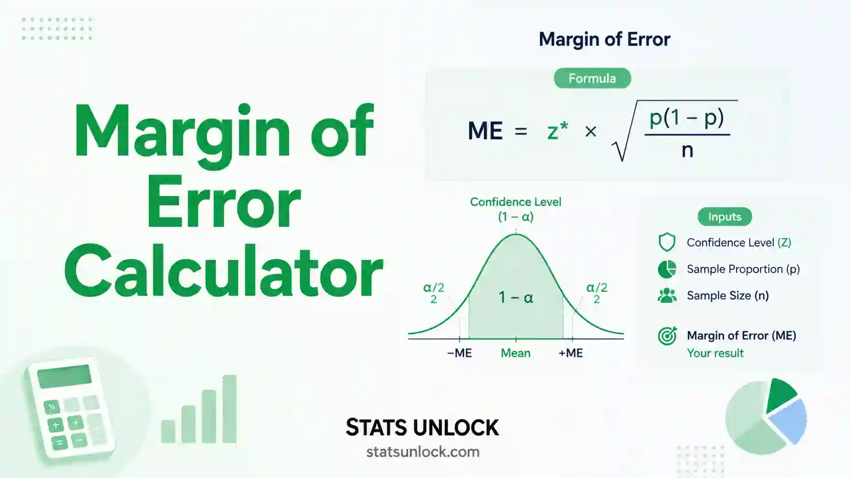

Margin of Error Calculator
Work out the margin of error for a survey percentage or a mean, run it backwards from a confidence interval, or find the sample size you need to hit a target. Includes the finite population correction, the Wilson interval for small percentages, and the design effect for cluster samples.
⚡ 0. Quick Answer
The margin of error is half the width of a confidence interval. It is the plus-or-minus figure you see after a poll result, and it answers one question: how far from the true value could this estimate plausibly be, given that you surveyed a sample rather than everybody?
📊 For a percentage (surveys, polls)
MOE = z × √[ p(1−p) / n ]A poll of 1,000 people showing 50% support has a margin of error of ±3.10 percentage points at 95% confidence. That is where the familiar "plus or minus three points" comes from.
📏 For an average (measurements)
MOE = t × (s / √n)Use t rather than z because you estimated the standard deviation from your data. A sample of 12 with a mean of 53.17 and an SD of 5.67 gives a margin of error of ±3.60.
MOE = (upper − lower) ÷ 2. An interval of 49.56 to 56.77 has a margin of error of 3.60. The From a confidence interval tab does this and recovers the standard error and sample size too.Key takeaways
- Margin of error scales with the square root of n. To halve it you must quadruple your sample. Going from 1,000 to 2,000 respondents only improves ±3.10 to ±2.19.
- Population size barely matters. A sample of 1,000 gives roughly ±3% whether the population is 50,000 or 50 million. This surprises almost everyone, and it is why national polls are not enormous.
- Use p = 0.5 when you do not know the proportion. That is the worst case and gives the widest margin, which is why survey firms quote it before fieldwork begins.
- The three numbers worth memorising: at 95% confidence you need about 385 people for ±5%, 1,068 for ±3% and 9,604 for ±1%.
- The quoted margin of error covers sampling error only. It says nothing about biased question wording, people who refused to answer, or a sampling frame that missed part of the population. Those are usually the larger problems.
- For percentages near 0% or 100% the standard formula breaks. At 2 out of 100 it produces a negative lower bound. Use the Wilson interval instead, which this calculator reports automatically.
📚 1. What Is the Margin of Error?
1.1 The idea in one paragraph
You want to know what a whole population thinks, but you can only afford to ask some of them. Whatever number your sample returns will be a little off, purely because you happened to ask these particular people rather than a different set. The margin of error quantifies how far off it could plausibly be. Ask more people and it shrinks; ask fewer and it grows.
1.2 Its exact relationship to the confidence interval
The margin of error and the confidence interval are the same information written two ways:
confidence interval = estimate ± margin of errorSo if a poll reports 52% with a margin of error of 3 points, the 95% confidence interval is 49% to 55%. Going the other way, if a paper reports an interval of 49% to 55%, the margin of error is (55 − 49) ÷ 2 = 3 points. Neither contains information the other lacks, which is why you can always convert between them.
1.3 What "95% confidence" actually means
It does not mean there is a 95% probability that the true value lies in this particular interval. The true value is a fixed number; it is either in there or it is not. What it means is that the procedure works 95% of the time: if you repeated the whole survey many times and built an interval each time, about 95 out of every 100 of those intervals would contain the true value.
In practice most people treat it as "we are fairly confident the truth is in this range", which is close enough for everyday use. The distinction matters when you start making probability statements about a specific interval, which is a Bayesian claim requiring different machinery.
1.4 The three levers
| What you change | Effect on the margin of error | How much |
|---|---|---|
| Increase the sample size | Shrinks it | By the square root. Quadrupling n halves the margin |
| Raise the confidence level | Widens it | 90% uses z = 1.645, 95% uses 1.960, 99% uses 2.576 |
| Move the proportion away from 50% | Shrinks it | p = 0.5 is the worst case. At p = 0.1 the margin is 40% smaller |
| Increase the population size | Almost nothing | Only matters when your sample is a large fraction of the population |
That last row is the counterintuitive one. Once the population is large relative to the sample, its exact size drops out of the arithmetic almost entirely. A sample of 1,000 gives a margin of about 3.1 points whether you are surveying a city of 50,000 or a country of 50 million. What matters is how many people you asked, not what fraction of the population they represent.
1.5 When population size does matter
If your sample is more than about 5% of the population, the finite population correction kicks in and shrinks the margin, because you are getting closer to a census. Surveying 1,000 people out of 5,000 gives ±2.77% rather than ±3.10%. Surveying 4,900 out of 5,000 gives a margin near zero, which is correct: you have nearly asked everybody.
FPC = √[ (N − n) / (N − 1) ]This is why an internal survey of a 200-person company needs far fewer responses than a national poll to reach the same precision.
1.6 What the margin of error does not cover
This is the most important paragraph on the page. The quoted margin of error accounts for random sampling error only. It assumes you drew a genuine random sample from exactly the population you meant to study, that everyone responded, and that they answered honestly and understood the question.
In real surveys the larger errors are usually elsewhere: people who could not be reached, people who refused, a sampling frame that excluded part of the population, leading question wording, and the choices made when weighting the data. None of these appear in the ± figure. A poll with a stated margin of ±3 points can easily be off by considerably more, and historically most large polling misses have come from these sources rather than from sampling error.
🧮 2. Set Up Your Calculation
📁 Or upload a CSV / Excel file
The classic survey case. Enter the percentage your sample reported and how many people you asked.
If you only have the published summary statistics, enter them here. This is the usual situation when checking a figure in a paper or a report.
Work backwards from a published interval. The margin of error is half its width, and the calculator also recovers the point estimate, the standard error and the sample size that must have produced it.
The planning calculation. Tell it how precise you need to be, and it tells you how many responses to collect.
📊 3. Results
🧠 4. Interpretation of Results, In Detail
4.1 What the plus-or-minus figure is claiming
When a poll reports 52% with a margin of error of 3 points, it is saying that the procedure used would capture the true population figure about 95 times out of 100, and that on this occasion it produced the range 49% to 55%. The true value is a fixed number, not a random one; what varies from survey to survey is the interval.
The practical reading is: the truth is plausibly anywhere between 49% and 55%, and values near the middle are more likely than values near the edges. That last point is often forgotten. The interval is not a uniform band where every value is equally credible; the estimate at the centre is the single most likely value and the plausibility falls away towards the limits.
4.2 The square root law, and why precision is expensive
The margin of error is proportional to one over the square root of n. This has consequences that surprise people who expect a linear relationship:
- Doubling your sample improves the margin by only about 29%, not 50%.
- To halve the margin you must quadruple the sample.
- Going from 1,000 to 2,000 respondents takes you from ±3.10% to ±2.19%. Going from 1,000 to 4,000 takes you to ±1.55%.
- The first few hundred responses buy you enormous precision; the next few thousand buy comparatively little.
This is why professional surveys cluster around 1,000 to 1,500 respondents. That is roughly where the curve flattens and additional fieldwork stops being worth the money.
4.3 Why the population size hardly matters
Almost everyone assumes a bigger population needs a bigger sample. It does not. A sample of 1,000 gives a margin of about ±3.1 points whether the population is 50,000 or 50 million, and the formula shows why: N does not appear in it at all unless the sample is a large fraction of the population.
The intuition is that you are measuring the composition of the population, not counting it. A well-stirred pot needs one spoonful to taste, whether the pot holds a litre or a hundred litres. What matters is that the stirring was thorough, which in survey terms means the sample was genuinely random.
The exception is when your sample is a meaningful share of the population, say above 5%. Then the finite population correction reduces the margin, because each person you sample removes some of the remaining uncertainty. Survey 1,000 out of 5,000 and the margin falls from 3.10% to 2.77%. Survey 4,900 out of 5,000 and it collapses to almost nothing, correctly: you have nearly conducted a census.
4.4 Why p = 0.5 is the worst case
The quantity p(1 − p) is largest at p = 0.5, where it equals 0.25, and it falls away symmetrically towards both extremes. At p = 0.1 it is 0.09, and the margin is about 40% smaller than at 50%.
This is why survey firms quote their headline margin at 50%: it is the widest the margin can be, so no result in the survey can be less precise than the quoted figure. It also means the margin reported for a whole survey applies exactly only to questions where the split is near even. A question where 90% agreed has a substantially tighter margin than the headline suggests.
4.5 Comparing two numbers, and the mistake journalists make
Suppose a poll with a margin of ±3 points shows Candidate A on 48% and Candidate B on 45%. Is A ahead? Almost certainly not in any statistically meaningful sense.
The margin applies to each estimate separately, and the difference between two estimates carries more uncertainty than either one alone. As a rough rule, the gap must exceed about twice the margin of error before you can be reasonably confident it is real. With a ±3 point margin, a 3-point lead is well inside the noise. Describing it as a lead, or worse as a "narrowing" lead compared with last month, is reading structure into randomness.
For proportions from the same survey the correct calculation is slightly more forgiving than doubling, because the two shares are negatively correlated, but doubling is a safe and simple heuristic that will keep you out of trouble.
4.6 When the standard formula breaks down
The usual formula is a normal approximation, and it fails when the percentage is close to 0% or 100%. Take 2 out of 100: the formula gives a margin of 2.74 points and an interval of −0.74% to 4.74%. A negative percentage is impossible, which tells you the method has broken.
Worse, at exactly 0 out of 50 the formula gives a margin of exactly zero, implying perfect certainty that nobody in the entire population holds that view, on the basis of 50 interviews. That is obviously absurd.
The Wilson score interval solves both problems. It is derived by inverting the test rather than approximating the estimate, cannot produce impossible values, and performs better than the standard interval at essentially all sample sizes. For 2 out of 100 it gives 0.55% to 7.00%, which is both possible and sensible. This calculator reports it alongside the standard interval every time, and where the two disagree you should use Wilson.
4.7 t or z, and why it matters for means
For a percentage the calculator uses z, the normal critical value. For a mean it uses t, because you almost always estimated the standard deviation from the same sample you are describing, and that estimate carries its own uncertainty.
The difference is largest at small n. At n = 5 the t critical value is 2.776 against the normal 1.960, so the margin is 42% wider. At n = 30 it is 2.045, only 4% wider. By n = 100 the gap is under 1%. Using z with a small sample understates your uncertainty, which is the more dangerous direction to err.
4.8 The design effect, for anything other than simple random sampling
The standard formula assumes every member of the population had an equal, independent chance of selection. Real surveys rarely work that way. They cluster by household, school, village or postcode, because sending an interviewer to one street is far cheaper than sending them to thirty scattered addresses.
Clustering costs precision, because people in the same cluster resemble each other, so each additional interview within a cluster adds less new information. The design effect quantifies that loss. A design effect of 2 means your survey carries the same sampling error as a simple random sample of half the size, so 1,000 clustered interviews behave like 500 independent ones. Typical values run from 1.5 to 3. Ignoring it will make your reported margin look considerably better than it is.
4.9 Reading the four charts
Chart 1 draws your interval with the estimate marked, which is the quickest way to see whether it crosses a threshold you care about. Chart 2 plots the margin against sample size and shows the square root law directly: the curve is steep at the left and almost flat by the right. Chart 3 shows how the margin varies with the percentage, peaking at 50%. Chart 4 shows what raising your confidence level costs you in precision.
Chart 2 is the one worth showing a client who is asking for a tighter number. It makes the cost of precision visible in a way that a table of figures does not.
4.10 The limitation that matters most
Everything on this page addresses random sampling error: the fact that you asked some people rather than all of them. It assumes you drew a genuine random sample from exactly the population you meant to study, that everybody responded, and that they understood and answered honestly.
Real surveys fail these assumptions routinely. Response rates for telephone polling have fallen into the single digits in many countries, and the people who still answer are not a random subset of those who do not. Online panels over-represent the engaged. Question wording nudges answers. Weighting corrects some of this and introduces assumptions of its own.
None of that appears in the ± figure. The margin of error is a statement about arithmetic under ideal conditions, and it should be read as a lower bound on your total uncertainty rather than a full accounting of it. When large surveys have been badly wrong, the failure has almost always been here rather than in the sampling error.
✍ 5. How to Write Your Results in Research
▶ Run the analysis above to auto-fill all five examples with your results.
📌 Key conventions for this style
- Always state the confidence level. A margin of error without one is meaningless.
- Give the sample size, because readers cannot judge precision without it.
- Use "percentage points" not "percent" for a margin on a percentage. A 3-point margin on 52% is not 3% of 52.
- Report the interval as well as the margin. They carry the same information but readers differ in which they find clearer.
📌 Key conventions for this style
- For tables, figure captions and parenthetical use.
- Keep the confidence level and n even when compressing.
- Define the format once in a footnote and use it consistently throughout.
📌 Key conventions for this style
- Avoid "margin of error", "confidence interval" and "statistically significant" entirely.
- "Probably between X and Y" is honest and understood by everyone.
- Never present a single number as if it were exact.
- Resist describing differences smaller than twice the margin as real.
📌 Key conventions for this style
- State the formula, the critical value and any corrections applied.
- Declare the design effect if the sample was not a simple random sample.
- Say explicitly that the margin excludes non-sampling error. Reviewers and standards bodies expect this.
- The AAPOR transparency initiative asks for the sampling frame, the response rate and the weighting scheme alongside the margin.
📌 Key conventions for this style
- Useful in a proposal, where the client wants to know what more money would buy.
- Quantify the square root law rather than describing it: give the actual n for a halved margin.
- Note that reducing the standard deviation through better measurement is often cheaper than increasing n.
- For subgroup analysis, warn that a subgroup of a quarter the size has double the margin.
∑ 6. Formulas Used
half-width = z√[ p(1−p)/n + z²/4n² ] ÷ (1 + z²/n)
📝 7. How to Use This Calculator
- Paste your numbers into the data column. Mean from raw data opens first, with one column ready to go. Enter your values comma-separated exactly as the placeholder shows, and the calculator works out the mean, standard deviation, standard error and degrees of freedom, then applies the t critical value because your SD was estimated.
- Or switch tab if you have something else. Survey percentage is the classic poll case. Mean from summary stats is for when you only have a published mean, SD and n. From a confidence interval works backwards from an interval you already have. Sample size I need is the planning calculation to run before collecting anything.
- Load a sample dataset to see how it behaves. Eight are built in, including a skewed income set that triggers the normality warning and a set of very tight measurements where the margin is tiny. Selecting one replaces the data column immediately.
- Add clusters to compare groups. Each gets its own margin of error and confidence interval. Every column has its own Clear and Remove button, and Remove is disabled on the last remaining column. You can also upload a CSV or Excel file and click the columns you want.
- For a survey percentage, enter the result and the sample size. You can type 52 or 0.52, both are understood. If you do not yet know the percentage, leave it at 50, which is the worst case and gives the widest, safest margin.
- Add clusters to compare groups. Each gets its own margin of error and interval. Every column has its own Clear and Remove button, and Remove is disabled on the last remaining column. You can also upload a CSV or Excel file and click the columns you want.
- To reverse-engineer a published result, use the confidence interval tab. Enter the two limits and the calculator returns the margin, the point estimate, and, if you supply the sample size, the standard error and standard deviation behind them.
- To plan a study, use the sample size tab. Tell it the margin you need and it tells you how many responses to collect, adjusted for the design effect, the population size and your expected response rate.
- Choose your confidence level deliberately. 95% is the convention, but it is only a convention. Higher confidence always means a wider margin, and chart 4 shows exactly what it costs you.
- Read the warnings before the numbers. They will tell you if your percentage is too close to 0 or 100 for the standard formula, if the interval has run outside the possible range, or if your sample is too small for the normal approximation. Where the Wilson interval is reported and differs, use it.
📊 8. How to Calculate Margin of Error in Excel
Excel handles every part of this, though the one-call function CONFIDENCE.T only works for means. For proportions you assemble it from three functions. Below is the whole workflow in ten steps, each with a picture of what your sheet should look like.
NORM.S.INV for the z critical value, SQRT for the standard error, T.INV.2T for a mean's critical value, CONFIDENCE.T to do a mean in one call, and ROUNDUP for sample size planning.Step 1. Lay out the three inputs you actually have: the percentage as a decimal, the sample size, and the confidence level.
Step 2. NORM.S.INV converts the confidence level into the z critical value. At 95% it returns 1.959964, which is where the familiar 1.96 comes from.
Step 3. The standard error of a proportion. Note SQRT wraps the whole expression, not just n.
Step 4. Margin of error = z times the standard error. 0.030965 as a decimal, which is 3.0965 percentage points.
Step 5. The confidence interval is the estimate plus and minus the margin: 48.90% to 55.10%. Format these cells as percentages to read them directly.
Step 6. The finite population correction, for when your sample is a large share of the population. At n=1000 out of N=5000 it is 0.8945.
Step 7. The design effect widens the margin by its square root. A DEFF of 2 turns 3.10 points into 4.38.
Step 8. For a MEAN use T.INV.2T, not NORM.S.INV. At n=12 it gives 2.201 rather than 1.960, because the SD was estimated from the sample.
Step 9. CONFIDENCE.T does the whole thing in one call and returns 3.6027. Do NOT use CONFIDENCE.NORM, which assumes you know the population SD and gives too narrow a margin.
Step 10. Sample size for a target margin: =B4^2*B3*(1-B3)/B2^2 gives 1067.07, and ROUNDUP makes it 1068. Always round up, never down.
The formula cheat sheet
| What you want | Excel formula | Result for the worked example |
|---|---|---|
| z critical value | =NORM.S.INV(1-(1-0.95)/2) | 1.959964 |
| z, the shortcut | =NORM.S.INV(0.975) | 1.959964, same thing |
| Standard error of a proportion | =SQRT(p*(1-p)/n) | 0.015799 |
| MOE for a proportion | =NORM.S.INV(0.975)*SQRT(p*(1-p)/n) | 0.030965, so ±3.0965 points |
| MOE at the worst case | =NORM.S.INV(0.975)*SQRT(0.25/n) | ±3.0990 points at n = 1000 |
| Standard error of a mean | =STDEV.S(range)/SQRT(COUNT(range)) | 1.636902 |
| t critical value | =T.INV.2T(0.05,n-1) | 2.200985 at n = 12 |
| MOE for a mean | =CONFIDENCE.T(0.05,sd,n) | 3.602693 |
| MOE for a mean, long form | =T.INV.2T(0.05,n-1)*sd/SQRT(n) | 3.602693, identical |
| Lower limit | =estimate-MOE | 49.5640 |
| Upper limit | =estimate+MOE | 56.7694 |
| MOE from a confidence interval | =(upper-lower)/2 | 3.6027 |
| Estimate from an interval | =(upper+lower)/2 | 53.1667 |
| Finite population correction | =SQRT((N-n)/(N-1)) | 0.894517 at n = 1000, N = 5000 |
| Design effect adjustment | =MOE*SQRT(deff) | 0.043791 at DEFF = 2 |
| Sample size for a proportion | =ROUNDUP(NORM.S.INV(0.975)^2*0.25/target^2,0) | 1068 for ±3% |
| Sample size for a mean | =ROUNDUP(NORM.S.INV(0.975)^2*sd^2/target^2,0) | 124 for ±1 with sd 5.67 |
| Sample size, finite population | =ROUNDUP(n/(1+(n-1)/N),0) | 880 for ±3% within N = 5000 |
| Wilson lower limit | =(p+z^2/(2*n)-z*SQRT(p*(1-p)/n+z^2/(4*n^2)))/(1+z^2/n) | 0.005502 for 2 out of 100 |
| Wilson upper limit | =(p+z^2/(2*n)+z*SQRT(p*(1-p)/n+z^2/(4*n^2)))/(1+z^2/n) | 0.070012 for 2 out of 100 |
Six mistakes that catch people out
- Using CONFIDENCE.NORM instead of CONFIDENCE.T. The NORM version assumes the population standard deviation is known and gives a margin that is too narrow. At n = 12 it returns 3.208 rather than the correct 3.603, understating your uncertainty by 11%.
- Putting SQRT in the wrong place. It must wrap the whole fraction:
SQRT(p*(1-p)/n), notSQRT(p*(1-p))/n. The second gives a completely different and much smaller number. - Feeding NORM.S.INV the confidence level directly.
NORM.S.INV(0.95)returns 1.645, the one-tailed value. For a two-sided margin you needNORM.S.INV(0.975). - Entering the percentage as 52 instead of 0.52. The formula needs a decimal. Using 52 gives a nonsensical negative value under the square root.
- Rounding sample size down. 1067.07 becomes 1068, not 1067. Use
ROUNDUP, notROUND, or you will fall just short of your target precision. - Applying the FPC when it does not apply. If your sample is under about 5% of the population the correction is nearly 1 and adds nothing but a chance to make an error.
NORMSINV, TINV and CONFIDENCE names. Note that legacy CONFIDENCE is the NORM version, so prefer CONFIDENCE.T explicitly.📈 9. How to Calculate Margin of Error in R
Base R does all of this with qnorm(), qt() and arithmetic. No packages are needed. The script below covers proportions, means, the reverse calculation from a confidence interval, sample size planning and the Wilson interval, then draws one figure.
prop.test() returns a Wilson interval with a continuity correction by default, not the textbook interval, so its limits will not equal p ± MOE. That is a feature rather than a bug, but it means you cannot read a margin of error straight off it. Use binom.test() for an exact Clopper-Pearson interval, or compute the standard margin yourself as shown below.# Margin of Error Calculator in R (base R, no packages)
conf <- 0.95
z <- qnorm(1 - (1 - conf)/2) # 1.959964 at 95%
# ---- 1. Margin of error for a survey percentage -----------------------
p <- 0.52; n <- 1000
se_p <- sqrt(p * (1 - p) / n)
moe_p <- z * se_p
# Finite population correction, only matters if n is a big share of N
N <- 5000
fpc <- sqrt((N - n) / (N - 1))
moe_fpc <- moe_p * fpc
# Design effect, for cluster or multistage samples
deff <- 2
moe_deff <- moe_p * sqrt(deff)
# ---- 2. Margin of error for a mean ------------------------------------
x <- c(52,48,55,61,47,58,50,63,45,56,54,49)
nm <- length(x)
m <- mean(x)
s <- sd(x) # sd() always divides by n - 1
se_m <- s / sqrt(nm)
tcrit <- qt(1 - (1 - conf)/2, nm - 1) # t, not z: s was estimated
moe_m <- tcrit * se_m
# t.test() gives the same interval, which is a useful cross-check
ci <- t.test(x, conf.level = conf)$conf.int
# ---- 3. Margin of error FROM a confidence interval --------------------
lo <- 49.5640; hi <- 56.7694
moe_ci <- (hi - lo) / 2
est_ci <- (hi + lo) / 2
se_back <- moe_ci / tcrit # recover SE, if you know n
sd_back <- se_back * sqrt(nm) # recover SD
# ---- 4. Sample size for a target margin -------------------------------
n_for_moe <- function(target, p = 0.5, conf = 0.95, N = NULL, deff = 1) {
z <- qnorm(1 - (1 - conf)/2)
n <- z^2 * p * (1 - p) / target^2
n <- n * deff
if (!is.null(N)) n <- n / (1 + (n - 1) / N) # finite population
ceiling(n)
}
# ---- 5. Wilson interval, for percentages near 0 or 100 ----------------
wilson <- function(k, n, conf = 0.95) {
z <- qnorm(1 - (1 - conf)/2)
p <- k / n
d <- 1 + z^2 / n
c <- (p + z^2 / (2*n)) / d
h <- z * sqrt(p*(1-p)/n + z^2/(4*n^2)) / d
c(max(0, c - h), min(1, c + h))
}
cat(sprintf("PROPORTION %.0f%% of n=%d: MOE = +/- %.4f pp\n", p*100, n, moe_p*100))
cat(sprintf(" interval %.2f%% to %.2f%%\n", (p-moe_p)*100, (p+moe_p)*100))
cat(sprintf(" with FPC N=%d: MOE = +/- %.4f pp (fpc %.6f)\n", N, moe_fpc*100, fpc))
cat(sprintf(" with DEFF deff=%g: MOE = +/- %.4f pp\n", deff, moe_deff*100))
cat(sprintf("MEAN n=%d, mean=%.4f, s=%.4f, SE=%.4f\n", nm, m, s, se_m))
cat(sprintf(" t(%d) = %.6f, MOE = +/- %.4f\n", nm-1, tcrit, moe_m))
cat(sprintf(" interval %.4f to %.4f\n", m-moe_m, m+moe_m))
cat(sprintf("FROM CI [%g, %g] -> MOE = +/- %.4f, estimate %.4f\n",
lo, hi, moe_ci, est_ci))
cat(sprintf(" recovered SE %.6f, SD %.6f\n", se_back, sd_back))
cat(sprintf("SAMPLE SIZE +/-5%%: %d +/-3%%: %d +/-1%%: %d\n",
n_for_moe(0.05), n_for_moe(0.03), n_for_moe(0.01)))
cat(sprintf(" +/-3%% within a population of 5000: %d\n",
n_for_moe(0.03, N = 5000)))
w <- wilson(2, 100)
cat(sprintf("WILSON 2/100: %.4f%% to %.4f%%\n", w[1]*100, w[2]*100))
cat(sprintf(" standard 2/100: %.4f%% to %.4f%% <- impossible lower bound\n",
(0.02 - z*sqrt(.02*.98/100))*100, (0.02 + z*sqrt(.02*.98/100))*100))
# ---- 6. One figure ----------------------------------------------------
ns <- seq(50, 5000, by = 10)
plot(ns, z*sqrt(0.5*0.5/ns)*100, type = "l", lwd = 2, col = "#0369a1",
ylim = c(0, 8), bty = "n", xlab = "sample size",
ylab = "margin of error (percentage points)",
main = sprintf("Margin of Error vs Sample Size at %.0f%% Confidence", conf*100))
lines(ns, z*sqrt(0.3*0.7/ns)*100, lwd = 2, col = "#0f766e")
lines(ns, z*sqrt(0.1*0.9/ns)*100, lwd = 2, col = "#b45309")
abline(v = c(385, 1068), col = "#94a3b8", lty = 3)
text(385, 7.6, " n=385\n +/-5%", pos = 4, cex = 0.75, col = "#64748b")
text(1068, 7.6, " n=1068\n +/-3%", pos = 4, cex = 0.75, col = "#64748b")
points(n, moe_p*100, pch = 19, cex = 1.4, col = "#be185d")
legend("topright", bty = "n", cex = 0.85,
legend = c("p = 50%", "p = 30%", "p = 10%",
sprintf("your survey: n=%d, +/-%.2f pp", n, moe_p*100)),
col = c("#0369a1", "#0f766e", "#b45309", "#be185d"),
lwd = c(2, 2, 2, NA), pch = c(NA, NA, NA, 19))
What the script prints
PROPORTION   52% of n=1000: MOE = +/- 3.0965 pp
             interval 48.90% to 55.10%
  with FPC   N=5000: MOE = +/- 2.7699 pp  (fpc 0.894517)
  with DEFF  deff=2: MOE = +/- 4.3791 pp
MEAN         n=12, mean=53.1667, s=5.6702, SE=1.6369
             t(11) = 2.200985, MOE = +/- 3.6027
             interval 49.5640 to 56.7694
FROM CI      [49.564, 56.7694] -> MOE = +/- 3.6027, estimate 53.1667
             recovered SE 1.636858, SD 5.670242
SAMPLE SIZE  +/-5%: 385   +/-3%: 1068   +/-1%: 9604
             +/-3% within a population of 5000: 880
WILSON       2/100: 0.5502% to 7.0012%
  standard   2/100: -0.7439% to 4.7439%  <- impossible lower bound
These are the same numbers the Python script produces and the same numbers the calculator at the top of this page produces.
Line-by-line explanation
- Block 1 computes the proportion margin from first principles, then shows both adjustments. Notice the finite population correction pulls the margin down while the design effect pushes it up: they work in opposite directions and both are commonly forgotten.
- Block 2 uses
qt()rather thanqnorm()because the standard deviation came from the sample. Thet.test()call is there as a cross-check: its confidence interval should match your hand calculation exactly, and if it does not you have made an arithmetic error. - Block 3 is the reverse direction, and it is two lines of arithmetic. The recovery of the standard deviation only works if you know n and the confidence level the original authors used.
- Block 4 is written as a reusable function because you will want it repeatedly. Note the
ceiling(): sample sizes always round up. - Block 5 implements Wilson directly rather than calling
prop.test(), so you can see the arithmetic and control the continuity correction yourself. - Block 6 draws the single most useful figure in survey planning: the margin against sample size for three different proportions, with the ±5% and ±3% landmarks marked. The flatness of the curve past about n = 1,500 is the whole argument for why polls are the size they are.
Useful one-liners
| Task | R |
|---|---|
| z critical value | qnorm(0.975) |
| t critical value | qt(0.975, df) |
| MOE for a proportion | qnorm(0.975)*sqrt(p*(1-p)/n) |
| MOE for a mean | qt(0.975,n-1)*sd(x)/sqrt(n) |
| Confidence interval for a mean | t.test(x)$conf.int |
| MOE from a t.test result | diff(t.test(x)$conf.int)/2 |
| Wilson interval (with correction) | prop.test(52,100)$conf.int |
| Wilson without the correction | prop.test(52,100,correct=FALSE)$conf.int |
| Exact Clopper-Pearson interval | binom.test(52,100)$conf.int |
| Sample size for ±3% | ceiling(qnorm(0.975)^2*0.25/0.03^2) |
| Finite population correction | sqrt((N-n)/(N-1)) |
| Survey package, design-based SE | survey::svymean(~x, design) |
| Bootstrap interval | boot::boot.ci(boot(x, mean_fn, 2000)) |
🐍 10. How to Calculate Margin of Error in Python
NumPy and SciPy cover everything here. The script below was run before being published, so the output shown underneath is the real console output, not typed by hand.
np.std() defaults to ddof=0, the population divisor. Write ddof=1 for a sample standard deviation, or your margin will be slightly too narrow. Second, statsmodels.stats.proportion.proportion_confint defaults to method='normal', the textbook interval that fails near 0% and 100%. Pass method='wilson' instead.# Margin of Error Calculator in Python
# Proportions, means, reverse from a confidence interval, and sample size.
import numpy as np
import matplotlib
matplotlib.use("Agg")
import matplotlib.pyplot as plt
from scipy import stats
conf = 0.95
z = stats.norm.ppf(1 - (1 - conf)/2) # 1.959964 at 95%
# ---- 1. Margin of error for a survey percentage -----------------------
p, n = 0.52, 1000
se_p = np.sqrt(p * (1 - p) / n)
moe_p = z * se_p
# Finite population correction, only matters if n is a big share of N
N = 5000
fpc = np.sqrt((N - n) / (N - 1))
moe_fpc = moe_p * fpc
# Design effect, for cluster or multistage samples
deff = 2.0
moe_deff = moe_p * np.sqrt(deff)
# ---- 2. Margin of error for a mean ------------------------------------
x = np.array([52,48,55,61,47,58,50,63,45,56,54,49], dtype=float)
nm = x.size
mean = x.mean()
s = x.std(ddof=1) # ddof=1: sample SD
se_m = s / np.sqrt(nm)
tcrit = stats.t.ppf(1 - (1 - conf)/2, nm - 1) # t, not z: s was estimated
moe_m = tcrit * se_m
# ---- 3. Margin of error FROM a confidence interval --------------------
lo, hi = 49.5640, 56.7694
moe_ci = (hi - lo) / 2
est_ci = (hi + lo) / 2
se_back = moe_ci / tcrit # recover SE, if you know n
sd_back = se_back * np.sqrt(nm) # recover SD
# ---- 4. Sample size for a target margin -------------------------------
def n_for_moe(target, p=0.5, conf=0.95, N=None, deff=1.0):
z = stats.norm.ppf(1 - (1 - conf)/2)
n = z**2 * p * (1 - p) / target**2
n *= deff
if N: # finite population correction
n = n / (1 + (n - 1) / N)
return int(np.ceil(n))
# ---- 5. Wilson interval, for percentages near 0 or 100 ----------------
def wilson(k, n, conf=0.95):
z = stats.norm.ppf(1 - (1 - conf)/2)
p = k / n
d = 1 + z**2 / n
c = (p + z**2 / (2*n)) / d
h = z * np.sqrt(p*(1-p)/n + z**2/(4*n**2)) / d
return max(0.0, c - h), min(1.0, c + h)
print(f"PROPORTION {p:.0%} of n={n}: MOE = +/- {moe_p*100:.4f} pp")
print(f" interval {(p-moe_p)*100:.2f}% to {(p+moe_p)*100:.2f}%")
print(f" with FPC N={N}: MOE = +/- {moe_fpc*100:.4f} pp (fpc {fpc:.6f})")
print(f" with DEFF deff={deff}: MOE = +/- {moe_deff*100:.4f} pp")
print(f"MEAN n={nm}, mean={mean:.4f}, s={s:.4f}, SE={se_m:.4f}")
print(f" t({nm-1}) = {tcrit:.6f}, MOE = +/- {moe_m:.4f}")
print(f" interval {mean-moe_m:.4f} to {mean+moe_m:.4f}")
print(f"FROM CI [{lo}, {hi}] -> MOE = +/- {moe_ci:.4f}, estimate {est_ci:.4f}")
print(f" recovered SE {se_back:.6f}, SD {sd_back:.6f}")
print(f"SAMPLE SIZE +/-5%: {n_for_moe(0.05)} +/-3%: {n_for_moe(0.03)} "
f"+/-1%: {n_for_moe(0.01)}")
print(f" +/-3% within a population of 5000: {n_for_moe(0.03, N=5000)}")
print(f"WILSON 2/100: {wilson(2,100)[0]*100:.4f}% to {wilson(2,100)[1]*100:.4f}%")
print(f" standard 2/100: {(0.02-z*np.sqrt(.02*.98/100))*100:.4f}% to "
f"{(0.02+z*np.sqrt(.02*.98/100))*100:.4f}% <- impossible lower bound")
# ---- 6. One figure ----------------------------------------------------
fig, ax = plt.subplots(figsize=(9, 5))
ns = np.arange(50, 5001, 10)
for pp, col in [(0.5, "#0369a1"), (0.3, "#0f766e"), (0.1, "#b45309")]:
ax.plot(ns, z*np.sqrt(pp*(1-pp)/ns)*100, color=col, lw=2,
label=f"p = {pp:.0%}")
ax.scatter([n], [moe_p*100], s=90, color="#be185d", zorder=5,
label=f"your survey: n={n}, +/-{moe_p*100:.2f} pp")
for mk, lbl in [(385, "+/-5%"), (1068, "+/-3%")]:
ax.axvline(mk, color="#94a3b8", ls=":", lw=1.2)
ax.text(mk, 7.6, f" n={mk}\n {lbl}", fontsize=8, color="#64748b")
ax.set_xlabel("sample size")
ax.set_ylabel("margin of error (percentage points)")
ax.set_title(f"Margin of Error vs Sample Size at {conf:.0%} Confidence")
ax.set_ylim(0, 8)
ax.legend(frameon=False, fontsize=9)
ax.spines[["top", "right"]].set_visible(False)
fig.tight_layout()
fig.savefig("margin_of_error.png", dpi=150)
print("saved margin_of_error.png")
Actual output from running the script
PROPORTION   52% of n=1000: MOE = +/- 3.0965 pp
             interval 48.90% to 55.10%
  with FPC   N=5000: MOE = +/- 2.7699 pp  (fpc 0.894517)
  with DEFF  deff=2.0: MOE = +/- 4.3791 pp
MEAN         n=12, mean=53.1667, s=5.6702, SE=1.6369
             t(11) = 2.200985, MOE = +/- 3.6027
             interval 49.5640 to 56.7694
FROM CI      [49.564, 56.7694] -> MOE = +/- 3.6027, estimate 53.1667
             recovered SE 1.636858, SD 5.670242
SAMPLE SIZE  +/-5%: 385   +/-3%: 1068   +/-1%: 9604
             +/-3% within a population of 5000: 880
WILSON       2/100: 0.5502% to 7.0012%
  standard   2/100: -0.7439% to 4.7439%  <- impossible lower bound
Line-by-line explanation
- Block 1 computes the proportion margin, then shows both adjustments separately. The finite population correction multiplies the margin by 0.8945 and the design effect multiplies it by the square root of 2. They pull in opposite directions, and real surveys often need both.
- Block 2 uses
stats.t.ppfrather thanstats.norm.ppfbecause the standard deviation was estimated. At n = 12 that is 2.201 rather than 1.960, a 12% wider margin. - Block 3 is the reverse direction and it is two lines of arithmetic: half the width, and the midpoint. The recovery of the standard error and standard deviation requires knowing n and assuming the original authors used the same confidence level and distribution.
- Block 4 wraps the sample size calculation in a function with optional finite population and design effect arguments. Note
np.ceil: always round up. - Block 5 implements Wilson directly. The printed comparison makes the failure of the standard method obvious: for 2 out of 100 it produces a lower bound of −0.74%, a negative percentage.
- Block 6 draws the margin against sample size for three proportions, with the ±5% and ±3% landmarks marked. This is the figure to show anyone asking why the survey cannot simply be made more precise.
Useful one-liners
| Task | Python |
|---|---|
| z critical value | stats.norm.ppf(0.975) |
| t critical value | stats.t.ppf(0.975, df) |
| MOE for a proportion | stats.norm.ppf(.975)*np.sqrt(p*(1-p)/n) |
| MOE for a mean | stats.t.ppf(.975,n-1)*x.std(ddof=1)/np.sqrt(n) |
| Confidence interval for a mean | stats.t.interval(.95, n-1, mean, sem) |
| Standard error of the mean | stats.sem(x) |
| Wilson interval | proportion_confint(k, n, method='wilson') |
| Standard (Wald) interval | proportion_confint(k, n, method='normal') |
| Exact Clopper-Pearson | proportion_confint(k, n, method='beta') |
| Sample size for a proportion | samplesize_confint_proportion(p, half_length) |
| MOE from an interval | (hi - lo) / 2 |
| Bootstrap interval | stats.bootstrap((x,), np.mean).confidence_interval |
| Complex survey design | samplics or statsmodels survey tools |
stats.t.interval(0.95, 11, 53.1667, 1.6369) returns (49.5640, 56.7694), the same interval the hand calculation gives. If your manual arithmetic disagrees with SciPy, the usual culprit is ddof or using z where t belongs.📋 11. Reference Tables
11.1 Margin of error by sample size and confidence level
Computed at p = 50%, the worst case, so no result in a survey of that size can be less precise than the figure shown. This is the table survey firms use to quote a headline margin.
| Sample size | 90% | 95% | 99% | 99.9% |
|---|---|---|---|---|
| 10 | 26.01% | 30.99% | 40.73% | 52.03% |
| 25 | 16.45% | 19.60% | 25.76% | 32.91% |
| 50 | 11.63% | 13.86% | 18.21% | 23.27% |
| 75 | 9.50% | 11.32% | 14.87% | 19.00% |
| 100 | 8.22% | 9.80% | 12.88% | 16.45% |
| 150 | 6.72% | 8.00% | 10.52% | 13.43% |
| 200 | 5.82% | 6.93% | 9.11% | 11.63% |
| 250 | 5.20% | 6.20% | 8.15% | 10.41% |
| 300 | 4.75% | 5.66% | 7.44% | 9.50% |
| 384 | 4.20% | 5.00% | 6.57% | 8.40% |
| 400 | 4.11% | 4.90% | 6.44% | 8.23% |
| 500 | 3.68% | 4.38% | 5.76% | 7.36% |
| 600 | 3.36% | 4.00% | 5.26% | 6.72% |
| 750 | 3.00% | 3.58% | 4.70% | 6.01% |
| 1,000 | 2.60% | 3.10% | 4.07% | 5.20% |
| 1,068 | 2.52% | 3.00% | 3.94% | 5.03% |
| 1,200 | 2.37% | 2.83% | 3.72% | 4.75% |
| 1,500 | 2.12% | 2.53% | 3.33% | 4.25% |
| 2,000 | 1.84% | 2.19% | 2.88% | 3.68% |
| 2,500 | 1.64% | 1.96% | 2.58% | 3.29% |
| 3,000 | 1.50% | 1.79% | 2.35% | 3.00% |
| 4,000 | 1.30% | 1.55% | 2.04% | 2.60% |
| 5,000 | 1.16% | 1.39% | 1.82% | 2.33% |
| 10,000 | 0.82% | 0.98% | 1.29% | 1.65% |
11.2 Margin of error by sample size and the percentage itself
The margin is widest at 50% and narrows towards both extremes. A question where 90% agreed is considerably more precise than the survey's headline margin suggests.
| Sample size | p = 5% | p = 10% | p = 20% | p = 30% | p = 40% | p = 50% |
|---|---|---|---|---|---|---|
| 10 | 13.51% | 18.59% | 24.79% | 28.40% | 30.36% | 30.99% |
| 25 | 8.54% | 11.76% | 15.68% | 17.96% | 19.20% | 19.60% |
| 50 | 6.04% | 8.32% | 11.09% | 12.70% | 13.58% | 13.86% |
| 75 | 4.93% | 6.79% | 9.05% | 10.37% | 11.09% | 11.32% |
| 100 | 4.27% | 5.88% | 7.84% | 8.98% | 9.60% | 9.80% |
| 150 | 3.49% | 4.80% | 6.40% | 7.33% | 7.84% | 8.00% |
| 200 | 3.02% | 4.16% | 5.54% | 6.35% | 6.79% | 6.93% |
| 250 | 2.70% | 3.72% | 4.96% | 5.68% | 6.07% | 6.20% |
| 300 | 2.47% | 3.39% | 4.53% | 5.19% | 5.54% | 5.66% |
| 384 | 2.18% | 3.00% | 4.00% | 4.58% | 4.90% | 5.00% |
| 400 | 2.14% | 2.94% | 3.92% | 4.49% | 4.80% | 4.90% |
| 500 | 1.91% | 2.63% | 3.51% | 4.02% | 4.29% | 4.38% |
| 600 | 1.74% | 2.40% | 3.20% | 3.67% | 3.92% | 4.00% |
| 750 | 1.56% | 2.15% | 2.86% | 3.28% | 3.51% | 3.58% |
| 1,000 | 1.35% | 1.86% | 2.48% | 2.84% | 3.04% | 3.10% |
| 1,068 | 1.31% | 1.80% | 2.40% | 2.75% | 2.94% | 3.00% |
| 1,200 | 1.23% | 1.70% | 2.26% | 2.59% | 2.77% | 2.83% |
| 1,500 | 1.10% | 1.52% | 2.02% | 2.32% | 2.48% | 2.53% |
| 2,000 | 0.96% | 1.31% | 1.75% | 2.01% | 2.15% | 2.19% |
| 2,500 | 0.85% | 1.18% | 1.57% | 1.80% | 1.92% | 1.96% |
| 3,000 | 0.78% | 1.07% | 1.43% | 1.64% | 1.75% | 1.79% |
| 4,000 | 0.68% | 0.93% | 1.24% | 1.42% | 1.52% | 1.55% |
| 5,000 | 0.60% | 0.83% | 1.11% | 1.27% | 1.36% | 1.39% |
| 10,000 | 0.43% | 0.59% | 0.78% | 0.90% | 0.96% | 0.98% |
11.3 Sample size needed for a target margin of error
The planning table. Read down to the precision you need and across to your confidence level. Assumes p = 50% and a very large population.
| Target margin | 90% confidence | 95% confidence | 99% confidence |
|---|---|---|---|
| ±10% | 68 | 97 | 166 |
| ±7% | 139 | 196 | 339 |
| ±5% | 271 | 385 | 664 |
| ±4% | 423 | 601 | 1,037 |
| ±3% | 752 | 1,068 | 1,844 |
| ±2.5% | 1,083 | 1,537 | 2,654 |
| ±2% | 1,691 | 2,401 | 4,147 |
| ±1.5% | 3,007 | 4,269 | 7,373 |
| ±1% | 6,764 | 9,604 | 16,588 |
| ±0.5% | 27,056 | 38,415 | 66,349 |
11.4 Sample size needed, by population size
This is the table that demonstrates how little population size matters. Look along the ±3% column: a population of 100,000 needs 1,056 responses and a population of 10 million needs 1,068. Twelve more people for a hundredfold larger population.
| Population size | ±10% | ±5% | ±3% | ±1% |
|---|---|---|---|---|
| 50 | 34 | 45 | 48 | 50 |
| 100 | 50 | 80 | 92 | 99 |
| 250 | 70 | 152 | 203 | 244 |
| 500 | 81 | 218 | 341 | 476 |
| 1,000 | 88 | 278 | 517 | 906 |
| 2,500 | 93 | 334 | 749 | 1,984 |
| 5,000 | 95 | 357 | 880 | 3,289 |
| 10,000 | 96 | 370 | 965 | 4,900 |
| 50,000 | 96 | 382 | 1,045 | 8,057 |
| 100,000 | 96 | 383 | 1,056 | 8,763 |
| 1,000,000 | 97 | 384 | 1,066 | 9,513 |
| 10,000,000 | 97 | 385 | 1,067 | 9,595 |
| Infinite | 97 | 385 | 1,068 | 9,604 |
Population size only bites when it is small. A 500-person organisation needs 218 responses for ±5%, not 385, because the finite population correction is doing real work at that scale.
11.5 The square root law, made concrete
What you actually get for your money. All figures at p = 50% and 95% confidence.
| Sample size | Relative to 1,000 | Margin of error | Margin as % of the n = 1,000 margin |
|---|---|---|---|
| 250 | 0.25x | 6.198% | 200.0% |
| 500 | 0.5x | 4.383% | 141.4% |
| 1,000 | 1x | 3.099% | 100.0% |
| 2,000 | 2x | 2.191% | 70.7% |
| 4,000 | 4x | 1.549% | 50.0% |
| 9,000 | 9x | 1.033% | 33.3% |
| 16,000 | 16x | 0.775% | 25.0% |
Read the last row: to reach a quarter of the margin you need sixteen times the sample. This relationship is fixed by the mathematics and no amount of budget changes it.
11.6 When the finite population correction matters
A fixed sample of 200 drawn from populations of different sizes. The correction is substantial when your sample is a large share of the population and negligible otherwise.
| Population (N) | n = 200 is this % of N | FPC | Margin without FPC | Margin with FPC |
|---|---|---|---|---|
| 200 | 100.0% | 0.000000 | 6.930% | 0.000% |
| 500 | 40.0% | 0.775372 | 6.930% | 5.373% |
| 1,000 | 20.0% | 0.894875 | 6.930% | 6.201% |
| 2,000 | 10.0% | 0.948921 | 6.930% | 6.576% |
| 5,000 | 4.0% | 0.979894 | 6.930% | 6.790% |
| 10,000 | 2.0% | 0.989999 | 6.930% | 6.860% |
| 50,000 | 0.4% | 0.998008 | 6.930% | 6.916% |
Below about 5% sampling fraction the correction changes the margin by under 3% of its own value, which is why it is usually ignored for national surveys and always applied for organisational ones.
11.7 Where the standard formula fails, and Wilson rescues it
All at n = 100 except the first row, at 95% confidence. The highlighted rows are where the standard interval produces something impossible.
| Result | p | Standard (Wald) interval | Wilson interval | Verdict |
|---|---|---|---|---|
| 0/50 | 0.0% | 0.00% to 0.00% | 0.00% to 7.13% | Standard fails |
| 1/100 | 1.0% | -0.95% to 2.95% | 0.18% to 5.45% | Standard fails |
| 2/100 | 2.0% | -0.74% to 4.74% | 0.55% to 7.00% | Standard fails |
| 5/100 | 5.0% | 0.73% to 9.27% | 2.15% to 11.18% | Both fine |
| 10/100 | 10.0% | 4.12% to 15.88% | 5.52% to 17.44% | Both fine |
| 25/100 | 25.0% | 16.51% to 33.49% | 17.55% to 34.30% | Both fine |
| 50/100 | 50.0% | 40.20% to 59.80% | 40.38% to 59.62% | Both fine |
| 90/100 | 90.0% | 84.12% to 95.88% | 82.56% to 94.48% | Both fine |
| 98/100 | 98.0% | 95.26% to 100.74% | 93.00% to 99.45% | Standard fails |
| 100/100 | 100.0% | 100.00% to 100.00% | 96.30% to 100.00% | Standard fails |
Note the first and last rows especially. At 0 out of 50 the standard formula reports a margin of exactly zero, claiming certainty that nobody in the population holds that view on the basis of 50 interviews. Wilson correctly returns 0% to 7.13%.
11.8 Critical values by confidence level
| Confidence level | Alpha | z (two-sided) | Margin at n = 1,000, p = 50% | n needed for ±3% |
|---|---|---|---|---|
| 80% | 0.20 | 1.2816 | ±2.03% | 456 |
| 85% | 0.15 | 1.4395 | ±2.28% | 576 |
| 90% | 0.10 | 1.6449 | ±2.60% | 752 |
| 95% | 0.05 | 1.9600 | ±3.10% | 1,068 |
| 98% | 0.02 | 2.3263 | ±3.68% | 1,504 |
| 99% | 0.01 | 2.5758 | ±4.07% | 1,844 |
| 99.9% | 0.001 | 3.2905 | ±5.20% | 3,008 |
11.9 t versus z for means, and the small-sample penalty
| n | df | t at 95% | z at 95% | t is wider by |
|---|---|---|---|---|
| 3 | 2 | 4.3027 | 1.9600 | 119.5% |
| 5 | 4 | 2.7764 | 1.9600 | 41.7% |
| 10 | 9 | 2.2622 | 1.9600 | 15.4% |
| 12 | 11 | 2.2010 | 1.9600 | 12.3% |
| 20 | 19 | 2.0930 | 1.9600 | 6.8% |
| 30 | 29 | 2.0452 | 1.9600 | 4.3% |
| 50 | 49 | 2.0096 | 1.9600 | 2.5% |
| 100 | 99 | 1.9842 | 1.9600 | 1.2% |
| 500 | 499 | 1.9647 | 1.9600 | 0.2% |
| 1,000 | 999 | 1.9623 | 1.9600 | 0.1% |
Using z instead of t on a sample of 10 understates your margin by 15%. Above about n = 50 the difference stops mattering in practice, but there is never a penalty for using t.
11.10 Design effects you might encounter
| Design | Typical DEFF | Effective n from 1,000 interviews | Margin (p = 50%) |
|---|---|---|---|
| Simple random sample | 1.0 | 1,000 | ±3.10% |
| Stratified, proportionate | 0.9 to 1.0 | 1,000 to 1,111 | ±2.94% to 3.10% |
| Systematic from an ordered list | 1.0 to 1.2 | 833 to 1,000 | ±3.10% to 3.39% |
| Household cluster sample | 1.5 to 2.5 | 400 to 667 | ±3.79% to 4.90% |
| Two-stage cluster, large clusters | 2.0 to 4.0 | 250 to 500 | ±4.38% to 6.20% |
| Weighted online panel | 1.3 to 2.0 | 500 to 769 | ±3.53% to 4.38% |
A stratified sample can have a design effect below 1, which means it is more efficient than simple random sampling. Every other design listed here costs you precision.
11.11 The same calculation in five packages
| Task | Excel | R | Python | SPSS | Stata |
|---|---|---|---|---|---|
| z critical value | NORM.S.INV(0.975) | qnorm(.975) | stats.norm.ppf(.975) | IDF.NORMAL(.975,0,1) | invnormal(.975) |
| t critical value | T.INV.2T(0.05,df) | qt(.975,df) | stats.t.ppf(.975,df) | IDF.T(.975,df) | invttail(df,.025) |
| MOE for a mean | CONFIDENCE.T(.05,sd,n) | qt(.975,n-1)*sd/sqrt(n) | stats.t.ppf(.975,n-1)*sem | EXAMINE /CINTERVAL | ci means x |
| CI for a proportion | build it manually | prop.test(k,n) | proportion_confint(k,n) | CTABLES | ci proportions x |
| Wilson interval | build it manually | prop.test(k,n,correct=FALSE) | proportion_confint(k,n,method='wilson') | not built in | ci proportions x, wilson |
| Sample size | ROUNDUP(z^2*.25/t^2,0) | ceiling(qnorm(.975)^2*.25/t^2) | samplesize_confint_proportion | not built in | power oneproportion |
| Proportion CI default | none | Wilson + correction | Wald (normal) | Wald | Wald |
prop.test() gives a Wilson interval with a continuity correction, while Python's proportion_confint defaults to the plain Wald interval. The same data will give visibly different limits in the two languages, and R's are the better ones.💡 12. Eight Worked Examples
Every number below was computed with the calculator on this page and cross-checked against SciPy. Each example has its own colour and its own figure. Together they cover the five things people actually need: a poll, a mean, a reverse calculation, the cases where the standard formula fails, and the planning calculation.
Setup: A poll of 1,000 people finds 52% support. 95% confidence.
| Sample percentage | 52.00% |
|---|---|
| Sample size | 1,000 |
| z at 95% confidence | 1.959964 |
| Standard error | 0.015799 |
| Margin of error | ±3.0965 percentage points |
| Confidence interval | 48.90% to 55.10% |
| Wilson interval | 48.90% to 55.08% |
| Margin at the worst case, p = 50% | ±3.0990 points |
Reading it: This is the familiar "plus or minus three points". The interval runs from 48.90% to 55.10%, which straddles the 50% line marked in the figure. So this poll cannot establish that support is above half, even though the headline number is 52%. The Wilson interval agrees closely here because 52% is nowhere near an extreme.
Setup: 52, 48, 55, 61, 47, 58, 50, 63, 45, 56, 54, 49
| n | 12 |
|---|---|
| Mean | 53.1667 |
| Standard deviation | 5.6702 |
| Standard error | 1.636855 |
| t critical value at 95% confidence | 2.200985 |
| z for comparison | 1.959964 |
| Margin of error | ±3.6027 |
| Confidence interval | 49.5640 to 56.7694 |
| Margin if you wrongly used z | ±3.2082 |
| Relative margin | 6.78% of the estimate |
Reading it: For a mean you use t, not z, because the standard deviation was estimated from the same 12 numbers. At df = 11 that means 2.201 rather than 1.960, widening the margin from 3.208 to 3.603, a difference of 12%. The grey bar in the figure shows the too-narrow interval you would have got with z. On small samples that understatement is the more dangerous direction to err.
Setup: A paper reports a 95% confidence interval of 49.564 to 56.769 from a sample of 12.
| Lower limit | 49.5640 |
|---|---|
| Upper limit | 56.7694 |
| Interval width | 7.2054 |
| Margin of error | ±3.6027 |
| Point estimate, the midpoint | 53.1667 |
| t critical value at n = 12 | 2.200985 |
| Recovered standard error | 1.636858 |
| Recovered standard deviation | 5.670242 |
| n needed to halve this margin | 48 |
Reading it: This is two lines of arithmetic: the margin is half the width, and the estimate is the midpoint. What makes it useful is the recovery. Knowing n = 12, the critical value must have been 2.201, so the standard error was 1.6369 and the standard deviation 5.6702. You have just reconstructed the original analysis from a published interval, which is exactly what a meta-analysis needs. The caveat is that it only works for symmetric intervals.
Setup: A survey of 100 people finds 2 who report the outcome, so p = 2%.
| Result | 2 out of 100 |
|---|---|
| Sample percentage | 2.00% |
| Standard margin of error | ±2.7439 percentage points |
| Standard interval | -0.7439% to 4.7439% |
| The problem | a negative percentage is impossible |
| Wilson interval | 0.5502% to 7.0012% |
| n × p | 2.0, well below the rule-of-thumb minimum of 10 |
| n × (1 − p) | 98.0 |
Reading it: The standard formula gives a lower bound of minus 0.74%, which cannot happen. The normal approximation behind it assumes the sampling distribution is symmetric, and near a boundary it simply is not. The Wilson interval, shown as the second bar, returns 0.55% to 7.00%: possible, asymmetric and correct. The usual rule of thumb is that n times p and n times (1 minus p) should both exceed 10, and here the first is only 2. Whenever your percentage is below about 10% or above 90%, report Wilson.
Setup: A company with 500 employees gets 200 responses, split 50/50.
| Sample size | 200 |
|---|---|
| Population size | 500 |
| Sampling fraction | 40.0% |
| Margin without the correction | ±6.9295 points |
| Finite population correction | 0.775372 |
| Margin with the correction | ±5.3730 points |
| Reduction | 22.5% narrower |
| n needed for a 5-point margin, ignoring N | 385 |
| n needed for a 5-point margin within N = 500 | 218 |
Reading it: Here the population is small enough that the correction does real work. Surveying 200 of 500 people is a 40% sampling fraction, and the correction cuts the margin from 6.93 to 5.37 points, a 22% improvement for free. The grey bar shows what you would have reported by ignoring it. This is the one situation where population size genuinely matters, and it is exactly the situation most online calculators handle badly by omitting the field entirely.
Setup: A poll of 1,000 shows Candidate A on 48% and Candidate B on 45%.
| Candidate A | 48.00% ± 3.10 points |
|---|---|
| Candidate B | 45.00% ± 3.08 points |
| Observed gap | 3.00 percentage points |
| Margin on the difference | ±4.3699 percentage points |
| Gap needed before it means anything | about 4.4 points |
| Verdict | the lead is inside the noise |
| Rule of thumb | a gap must exceed roughly twice the individual margin |
Reading it: The two intervals overlap across almost their whole length, as the figure shows. The margin on a difference is larger than the margin on either estimate, here about 4.37 points, so a 3-point gap establishes nothing. Reporting this as a lead, or comparing it with last month's 2-point gap and calling it momentum, is reading structure into randomness. The practical rule is that a gap must exceed roughly twice the individual margin before you should describe it as real.
Setup: You need a margin of 3 percentage points at 95% confidence. How many people must you survey?
| Target margin | 3.00 percentage points |
|---|---|
| Confidence level | 95% |
| Assumed proportion | 50%, the worst case |
| Calculation | 1.959964 squared × 0.25 ÷ 0.03 squared |
| Unrounded result | 1067.072 |
| Sample size needed | 1,068 |
| For a 5-point margin instead | 385 |
| For a 1-point margin instead | 9,604 |
| At a 30% response rate | invite 3,560 people |
| With a design effect of 2 | 2,136 |
Reading it: The three landmark numbers are worth memorising: 385 for a 5-point margin, 1,068 for 3 points and 9,604 for 1 point. The figure shows why almost every commercial poll lands between 1,000 and 1,500. The curve is steep on the left, where each extra respondent buys real precision, and nearly flat on the right, where thousands more buy very little. Tightening from 3 points to 1 point requires nine times the sample and is rarely worth the cost.
Setup: A household cluster survey collects 1,000 interviews with a design effect of 2.0.
| Nominal sample size | 1,000 |
|---|---|
| Design effect | 2.0 |
| Effective sample size | 500 |
| Margin assuming simple random sampling | ±3.0990 points |
| Margin with the design effect | ±4.3826 points |
| Understatement if you ignore it | 41.4% |
| n needed for a 3-point margin with DEFF = 2 | 2,136 |
| Typical DEFF for household clusters | 1.5 to 3 |
Reading it: Clustering saves money and costs precision. Interviewing thirty households on one street is far cheaper than thirty scattered addresses, but neighbours resemble each other, so each extra interview within a cluster adds less new information. A design effect of 2 means these 1,000 interviews carry the same sampling error as 500 independent ones, widening the margin from 3.10 to 4.38 points. The grey bar is the figure you would have wrongly reported. Any survey that is not a simple random sample needs this adjustment, and omitting it is one of the most common errors in published survey work.
📋 13. Survey Design Protocol
The margin of error is the last thing you calculate and the first thing people quote. Everything that determines whether it means anything happens before a single response arrives.
- Define the target population precisely before anything else. "Adults in the region" is not a definition. Which adults, at what age boundary, resident how long, reachable by what means? The margin of error describes your uncertainty about this population, so if it is vague your result is vague.
- Choose the sample size in advance and write it down. Use the sample size tab. Collecting until the result looks convincing is the survey equivalent of optional stopping and destroys the meaning of the margin.
- Assume p = 0.5 when planning unless you have solid prior information. It is the worst case, so your realised margin can only be better than planned. Assuming 20% and finding 45% leaves you less precise than you promised.
- Build the sampling frame and document what it excludes. A telephone frame misses people without phones. An email list misses people who never signed up. These exclusions do not appear in the margin of error and are usually the larger problem.
- Randomise selection properly. The formula assumes every member of the population had a known, non-zero chance of selection. Convenience samples, self-selecting web polls and "whoever answered" have no defensible margin of error at all, however large they are.
- Record the design effect if you cluster. Sampling by household, school or postcode is cheaper and less precise. Estimate the design effect from a pilot or from comparable published surveys, and apply it to both your planning and your reporting.
- Plan for non-response and inflate the invitation list. A 30% response rate means inviting more than three times your target. Then record the actual rate, because it is a stronger signal of quality than the margin of error is.
- Pilot the questionnaire. Ambiguous wording produces measurement error that no sample size can fix. A pilot of thirty people will catch most of it.
- Decide the confidence level in advance and use the same one throughout. Reporting some results at 95% and others at 90% because it makes them look better is indefensible.
- Work out the margin for your smallest subgroup, not just the total. A survey of 1,000 with a 3-point margin gives a 6-point margin on a quarter of the sample and a 10-point margin on a tenth of it. Subgroup findings are far less precise than the headline, and this is the single most common way survey results are oversold.
- Keep the raw response file untouched. Do weighting and cleaning in a script so that every published figure can be traced back.
- Report the margin alongside the response rate, the frame and the weighting. The AAPOR transparency standards ask for all of these. A margin of error quoted alone is close to meaningless.
🎯 14. When to Use a Margin of Error, and When Not To
Use it when
- You have a genuine probability sample and want to express how precise your estimate is.
- You are reporting a survey percentage or a mean to an audience who will otherwise read the point estimate as exact.
- You are planning a study and need to justify a sample size to a client, a funder or an ethics committee.
- You want to know whether two numbers differ meaningfully. Compare the gap against roughly twice the margin.
- You are checking somebody else's work. A published interval yields the margin, and with n it yields the standard deviation too.
Do not use it when
- The sample was not random. Opt-in web polls, convenience samples and self-selected respondents have no valid margin of error. Reputable pollsters explicitly decline to quote one for non-probability panels.
- You measured the entire population. A census has no sampling error. If you surveyed all 40 employees, the answer is the answer.
- The interval is asymmetric. Wilson intervals, bootstrap intervals, and intervals for ratios, odds ratios or skewed quantities are deliberately not centred on the estimate. Report the limits instead.
- Your outcome is a median, a maximum or a rank. These have sampling distributions that are not symmetric or normal. Use a bootstrap.
- The percentage is very close to 0% or 100%. The standard formula gives impossible values. Use Wilson or an exact Clopper-Pearson interval.
- The main problem is bias, not sampling error. A margin of ±3 points on a survey with a 4% response rate is a precise measurement of a possibly unrepresentative group.
- You are comparing more than two groups. Looking at whether many pairs of intervals overlap inflates your error rate. Use a proper multiple comparison procedure.
What to use instead
| Situation | Better choice | Why |
|---|---|---|
| Percentage near 0 or 100 | Wilson score interval | Cannot produce impossible values |
| Very small counts | Clopper-Pearson exact interval | Guaranteed coverage, though conservative |
| Skewed data or a median | Bootstrap percentile interval | Makes no distributional assumption |
| Cluster or stratified design | Design-based standard errors | R's survey package, Stata's svy commands |
| Non-probability panel | A credibility interval, clearly labelled | Honest about the modelling assumptions involved |
| Comparing two groups | Margin on the difference | Larger than either individual margin |
| Many subgroups | Simultaneous confidence intervals | Controls the family-wise error rate |
| A rate or a count | Poisson confidence interval | Correct distribution for count data |
| Testing a specific hypothesis | A t-test or z-test | Gives a p-value, which an interval does not directly |
🔧 15. Troubleshooting
| Symptom | Cause | Fix |
|---|---|---|
| The interval runs below 0% or above 100% | Normal approximation failing near a boundary | Use the Wilson interval, which this calculator always reports |
| The margin came out as exactly zero | Your result was 0% or 100% | The standard formula is wrong here. Wilson gives a sensible interval |
| Your margin looks far too small | Entered the percentage as 52 rather than 0.52 in a formula | The formula needs a decimal. This calculator accepts either |
| Excel's answer is narrower than expected | Used CONFIDENCE.NORM instead of CONFIDENCE.T | The T version accounts for an estimated standard deviation |
| R and Python give different intervals for a proportion | R's prop.test uses Wilson with a correction; Python defaults to Wald | Pass method='wilson' in Python, or correct=FALSE in R |
| The margin barely changed when you doubled n | The square root law | Correct behaviour. Doubling n improves the margin by only 29% |
| Adding the population size did nothing | Your sample is under 5% of the population | Also correct. The FPC only matters at larger sampling fractions |
| Your subgroup result looks implausibly precise | Applied the whole-survey margin to a subgroup | Recompute using the subgroup's own n. A quarter of the sample doubles the margin |
| Two overlapping intervals were called significantly different | Compared the intervals rather than the difference | Compute the margin on the difference, or use a two-sample test |
| SQRT is giving an error or a strange result | Brackets in the wrong place | It is SQRT(p*(1-p)/n), with the whole fraction inside |
| NORM.S.INV returned 1.645 instead of 1.96 | Passed 0.95 rather than 0.975 | For a two-sided margin use NORM.S.INV(1-(1-conf)/2) |
| The reported margin seems too good for a cluster survey | Design effect ignored | Set it to 1.5 to 3 for a household cluster design |
| Your poll was outside its own margin of error | Non-sampling error: frame, non-response or wording | The margin never covered these. Report the response rate too |
| Sample size came out fractional | Normal, the formula is continuous | Always round up, never down |
| Reverse calculation gives an odd standard deviation | The source used a different confidence level or an asymmetric interval | Check the methods section before trusting the recovery |
| A 3% margin was described as "3% of the result" | Confusing percentage points with percent | ±3 points on 52% means 49% to 55%, not 50.4% to 53.6% |
⚖ 16. Assumptions and Limitations
What the margin of error assumes, ranked by how much it matters
| Assumption | How much it matters | What happens if it fails | How to check |
|---|---|---|---|
| Genuine random sampling | Critical | The margin becomes meaningless. No sample size repairs it | Not testable from the data. It is a property of the design |
| Everyone selected responded | Critical in practice | Respondents may differ systematically from non-respondents | Report the response rate and compare respondents against known population figures |
| The frame covers the population | Critical | Whole groups excluded, and no amount of data reveals it | Document what the frame excludes |
| Independent observations | High | Clustering makes the true margin wider than reported | Estimate the design effect |
| n×p and n×(1−p) both above 10 | Moderate | The normal approximation fails and the interval can go outside 0 to 100% | Multiply and check. The calculator warns you |
| Approximate normality (for means) | Moderate, falling as n grows | Inaccurate coverage below about n = 15 | Histogram, Q-Q plot, or use a bootstrap |
| The correct critical value | Moderate at small n | Using z instead of t understates the margin by 15% at n = 10 | Use t whenever the SD was estimated |
| Honest, consistent answers | Varies | Measurement error that the margin does not capture | Pilot the questionnaire |
Limitations worth stating whenever you publish a margin
- It covers sampling error only. This is the limitation that matters most and the one most often omitted. Non-response, coverage gaps, question wording and weighting decisions are all outside it, and in modern surveys they are usually larger.
- It assumes a probability sample. Opt-in panels and web polls have no valid margin of error regardless of size. Some organisations report a "credibility interval" instead, which is honest about the modelling assumptions involved.
- It applies to the whole sample, not to subgroups. A survey of 1,000 with ±3 points gives about ±6 points on a subgroup of 250 and ±10 on a subgroup of 100. Reporting subgroup findings under the headline margin is the most common way survey results get oversold.
- The quoted figure is usually the worst case. Computed at p = 50%, it overstates the margin for questions with lopsided answers.
- Comparing two estimates needs a different, larger margin. A gap must exceed roughly twice the individual margin before it is worth discussing.
- The confidence level is a convention. 95% has no special mathematical status. It was a convenience Fisher suggested and it stuck.
- The interval is not uniform. Values near the centre are considerably more plausible than values at the edges, which the flat ± notation hides.
- Repeated polling guarantees apparent movement. If you run twenty polls at 95% confidence, one will fall outside its interval by chance. Tracking studies routinely report this noise as a trend.
🏁 17. Conclusion
The margin of error is half the width of a confidence interval, and it exists because you asked some people rather than all of them. For a percentage it is z times the square root of p(1 − p) over n. For a mean it is t times the standard error. If you already have an interval, it is simply half the width, and if you also know the sample size you can work back to the standard error and the standard deviation behind it. That is the entire arithmetic, and it fits in a paragraph.
Three properties of that arithmetic surprise almost everyone. The first is the square root law: the margin falls with the square root of n, so doubling your sample improves precision by only 29% and halving the margin costs four times the sample. This is why commercial polls cluster between 1,000 and 1,500 respondents, and why a client asking to go from ±3 points to ±1 point is asking for a survey nine times the size.
The second is that population size barely matters. A sample of 1,000 gives about ±3.1 points whether the population is 50,000 or 50 million; the reference table shows a hundredfold increase in population changing the required sample by twelve people. What you are measuring is the composition of the population, not counting it, and a well-stirred pot needs one spoonful whatever its size. The exception is when your sample is a large share of the population, which is precisely the situation an internal company survey is in, and there the finite population correction does real work.
The third is that p = 0.5 is the worst case. That is why survey firms quote their headline margin at fifty per cent before fieldwork begins: nothing in the survey can turn out less precise than the number they promised.
Two failure modes are worth memorising. When a percentage sits close to 0% or 100%, the standard formula produces impossible results, including a negative lower bound for 2 out of 100 and a margin of exactly zero for 0 out of 50. The Wilson score interval fixes both and is never worse, so this calculator reports it every time. And when a survey is not a simple random sample, the design effect widens the margin: a household cluster design with a design effect of 2 means your thousand interviews carry the same sampling error as five hundred independent ones. Omitting it is one of the commonest errors in published survey work.
The most consequential limitation is not mathematical at all. The margin of error accounts for random sampling error and nothing else. It assumes a genuine random sample from exactly the population you meant to study, that everybody responded, and that they understood and answered honestly. Real surveys fail these assumptions routinely, response rates for telephone polling have collapsed into single digits in many countries, and the people who still answer are not a random subset of those who do not. None of that appears in the plus-or-minus figure. Treat it as a lower bound on your total uncertainty rather than a full accounting of it, and report the response rate, the sampling frame and the weighting scheme alongside it.
Finally, resist the most common misreading of all. Two estimates whose intervals overlap are not distinguishable, and a gap must exceed roughly twice the individual margin before it is worth discussing. A three-point lead in a poll with a three-point margin is not a lead. It is noise with a headline attached.
❓ 18. Frequently Asked Questions
What is the margin of error in simple terms?
How do you calculate margin of error?
How do I calculate margin of error from a confidence interval?
How is margin of error calculated in Excel?
=CONFIDENCE.T(0.05, standard_deviation, sample_size), which does the whole thing in one call. For a percentage there is no single function, so build it: =NORM.S.INV(0.975)*SQRT(p*(1-p)/n). Do not use CONFIDENCE.NORM for a mean, because it assumes the population standard deviation is known and gives a margin that is too narrow.What is a good margin of error?
What sample size do I need for a 5% margin of error?
Does the population size affect the margin of error?
Why does the margin of error use 50% when the result is different?
Does doubling my sample size halve the margin of error?
What is the difference between margin of error and standard error?
Should I use z or t for the margin of error?
Can the margin of error be larger than the result itself?
What is the Wilson interval and when should I use it?
Two poll results overlap. Are they different?
What is a design effect and do I need one?
Does the margin of error account for people who did not respond?
Can I quote a margin of error for an online or opt-in poll?
How does the confidence level change the margin?
Does the margin of error apply to subgroups too?
Is a margin of error of 3% the same as 3% of my result?
🔖 19. Cite This Tool
🔗 20. Related Calculators
📖 21. Glossary
| Term | Meaning |
|---|---|
| Margin of error | Half the width of a confidence interval. The plus-or-minus figure after an estimate. |
| Confidence interval | The estimate plus and minus the margin of error. Carries exactly the same information. |
| Confidence level | How often the procedure captures the true value across repeated samples. Conventionally 95%. |
| Standard error | The standard deviation of the sampling distribution. The margin before the critical value is applied. |
| Critical value | The multiplier, 1.96 for z at 95%, or a t value for a mean. |
| Sampling error | The variation that arises purely from surveying a sample rather than everybody. The only thing the margin covers. |
| Non-sampling error | Everything else: non-response, coverage gaps, question wording, measurement error. Not in the margin. |
| Coverage error | Error arising when the sampling frame does not include the whole target population. |
| Non-response bias | Error arising when the people who answer differ systematically from those who do not. |
| Sampling frame | The list from which the sample is actually drawn. |
| Probability sample | A sample where every member had a known, non-zero chance of selection. Required for a valid margin. |
| Convenience sample | A non-probability sample. Has no defensible margin of error at any size. |
| Finite population correction (FPC) | √[(N−n)/(N−1)]. Narrows the margin when the sample is a large share of the population. |
| Sampling fraction | n divided by N. The FPC matters once this exceeds about 5%. |
| Design effect (DEFF) | How much a complex design inflates the variance relative to simple random sampling. |
| Effective sample size | n divided by the design effect. What your clustered sample is really worth. |
| Cluster sampling | Sampling groups such as households or schools rather than individuals. Cheaper and less precise. |
| Stratified sampling | Dividing the population into strata and sampling within each. Can be more efficient than simple random sampling. |
| Wald interval | The standard textbook interval for a proportion. Fails near 0% and 100%. |
| Wilson score interval | A better interval for proportions that cannot produce impossible values. Asymmetric. |
| Clopper-Pearson interval | An exact interval for a proportion. Guaranteed coverage but conservative. |
| Credibility interval | The label used by some pollsters for non-probability panels, where a margin of error is not defensible. |
| Percentage point | The unit of a margin on a percentage. ±3 points on 52% means 49% to 55%. |
| Point estimate | The single best estimate, at the centre of a symmetric interval. |
| Weighting | Adjusting responses so the sample matches known population characteristics. Adds its own uncertainty. |
| Response rate | The proportion of those selected who provided a usable response. Often more informative about quality than the margin. |
| Bootstrap interval | An interval built by resampling. Useful for medians and skewed data where a symmetric margin is wrong. |
📚 22. References
- Wilson, E. B. (1927). Probable inference, the law of succession, and statistical inference. Journal of the American Statistical Association, 22(158), 209-212. doi.org/10.1080/01621459.1927.10502953
- Brown, L. D., Cai, T. T., & DasGupta, A. (2001). Interval estimation for a binomial proportion. Statistical Science, 16(2), 101-133. doi.org/10.1214/ss/1009213286
- Agresti, A., & Coull, B. A. (1998). Approximate is better than "exact" for interval estimation of binomial proportions. The American Statistician, 52(2), 119-126. doi.org/10.1080/00031305.1998.10480550
- Newcombe, R. G. (1998). Two-sided confidence intervals for the single proportion: comparison of seven methods. Statistics in Medicine, 17(8), 857-872. doi.org/10.1002/(SICI)1097-0258
- Clopper, C. J., & Pearson, E. S. (1934). The use of confidence or fiducial limits illustrated in the case of the binomial. Biometrika, 26(4), 404-413. doi.org/10.1093/biomet/26.4.404
- Cochran, W. G. (1977). Sampling Techniques (3rd ed.). Wiley. wiley.com
- Kish, L. (1965). Survey Sampling. Wiley. wiley.com
- Lohr, S. L. (2021). Sampling: Design and Analysis (3rd ed.). CRC Press. doi.org/10.1201/9780429298899
- Groves, R. M., et al. (2009). Survey Methodology (2nd ed.). Wiley. wiley.com
- Groves, R. M., & Peytcheva, E. (2008). The impact of nonresponse rates on nonresponse bias: A meta-analysis. Public Opinion Quarterly, 72(2), 167-189. doi.org/10.1093/poq/nfn011
- American Association for Public Opinion Research (2023). Standard Definitions: Final Dispositions of Case Codes and Outcome Rates for Surveys (10th ed.). aapor.org
- AAPOR Task Force (2013). Report on Non-Probability Sampling. American Association for Public Opinion Research. aapor.org
- Kennedy, C., et al. (2018). An Evaluation of the 2016 Election Polls in the United States. Public Opinion Quarterly, 82(1), 1-33. doi.org/10.1093/poq/nfx047
- Sturgis, P., et al. (2018). An assessment of the causes of the errors in the 2015 UK general election opinion polls. Journal of the Royal Statistical Society Series A, 181(3), 757-781. doi.org/10.1111/rssa.12329
- Cumming, G., & Finch, S. (2005). Inference by eye: Confidence intervals and how to read pictures of data. American Psychologist, 60(2), 170-180. doi.org/10.1037/0003-066X.60.2.170
- Greenland, S., et al. (2016). Statistical tests, p-values, confidence intervals, and power: A guide to misinterpretations. European Journal of Epidemiology, 31, 337-350. doi.org/10.1007/s10654-016-0149-3
- Neyman, J. (1937). Outline of a theory of statistical estimation based on the classical theory of probability. Philosophical Transactions of the Royal Society A, 236(767), 333-380. doi.org/10.1098/rsta.1937.0005
- Krejcie, R. V., & Morgan, D. W. (1970). Determining sample size for research activities. Educational and Psychological Measurement, 30(3), 607-610. doi.org/10.1177/001316447003000308
- Virtanen, P., et al. (2020). SciPy 1.0: Fundamental algorithms for scientific computing in Python. Nature Methods, 17, 261-272. doi.org/10.1038/s41592-019-0686-2
- Lumley, T. (2010). Complex Surveys: A Guide to Analysis Using R. Wiley. doi.org/10.1002/9780470580066