How is AIC used to compare GLM models?

Akaike Information Criterion (AIC) balances goodness-of-fit (log-likelihood) against model complexity (number of parameters). Lower AIC is better. A difference of >2 is meaningful; >10 is strong evidence the lower-AIC model fits better. BIC penalizes complexity more strongly than AIC.

What is overdispersion in count GLMs?

Overdispersion occurs when the observed variance exceeds the variance assumed by the model — most commonly when Poisson regression shows residual variance much greater than the mean. The dispersion ratio (Pearson χ² / residual df) should be near 1.0; values above ~1.5 suggest switching to Negative Binomial regression.

What sample size does a GLM need?

A common rule of thumb is at least 10 events per predictor (EPV) for logistic regression and 10–20 observations per parameter for Poisson and Gamma GLMs. Smaller samples produce unstable coefficients and unreliable standard errors. Use bias-corrected methods (Firth penalised likelihood) when events are rare.

Can I report this calculator's output in published research?

This tool is designed for teaching, exploratory analysis, and rapid prototyping. For peer-reviewed publication, validate the results in R (glm function, MASS::glm.nb), Python (statsmodels.api.GLM), or SPSS, and report: family, link, coefficients with 95% CI, exponentiated effects, AIC/BIC, null and residual deviance, and dispersion.

Generalized Linear Models (GLMs) Calculator | Free Online — Stats Unlock

Generalized Linear Models (GLMs) Calculator | Free Online GLM Tool — StatsUnlock

Statistical Models · GLM

Generalized Linear Models (GLMs)

Fit logistic, Poisson, Gamma, and Negative Binomial regression models with link functions, AIC/BIC, deviance, full coefficient tables, and four publication-quality diagnostic plots — all in your browser, free.

GLM Logistic Poisson Gamma Negative Binomial Link Functions AIC / BIC

1 · Data Input

Enter predictor cluster(s) and an outcome (Y). Three input methods supported.

Sample dataset

GLM family / link

Logit link · binary 0/1 outcome.

Outcome (Y) — comma-separated, default

Counts: 0 — values entered.

Upload CSV or Excel file (.csv, .txt, .xlsx, .xls)

Step 1 — choose Predictor (X) columns (one or more), then Step 2 — choose the single Outcome (Y) column. Headers auto-detected.

Manual entry mirrors the typed-data tab. Use the cluster fields above to type values directly. For larger datasets prefer the Upload tab.

Significance level (α)

Confidence level

5 · Technical Notes — formulas & conventions

Show formulas, link functions, and exponential-family identities

A GLM has three components: a random component (response distribution from the exponential family), a systematic component (linear predictor η = Xβ), and a link function g(·) joining them.

g(μ) = η = β₀ + β₁X₁ + β₂X₂ + … + βₚXₚ

Where: μ = E[Y|X]; g(·) is the link function; X are predictors; β are coefficients estimated by maximum likelihood (IRLS).

Logistic (Binomial · logit): log(μ/(1−μ)) = Xβ ⇒ μ = 1/(1+e^(−Xβ)) Poisson (log): log(μ) = Xβ ⇒ μ = e^(Xβ) Gamma (log): log(μ) = Xβ ⇒ μ = e^(Xβ), Var(Y) = φμ² Negative Binomial (log): log(μ) = Xβ ⇒ Var(Y) = μ + μ²/k Gaussian (identity): μ = Xβ ⇒ classical linear regression

Deviance: D = 2 × (ℓ_sat − ℓ_model) AIC: AIC = −2ℓ + 2p BIC: BIC = −2ℓ + p·ln(n) McFadden pseudo-R²: R²_M = 1 − (D_model / D_null) Dispersion ratio: φ̂ = Σ(Pearson residuals²) / (n − p)

Where: ℓ = log-likelihood; ℓ_sat = saturated model log-likelihood; p = number of parameters; n = sample size; D_null = deviance of intercept-only model.

Coefficient z-test: z = β̂ / SE(β̂), p = 2·(1 − Φ(|z|)) Wald 95% CI: β̂ ± 1.96·SE(β̂) Exponentiated CI: [exp(β̂ − 1.96·SE), exp(β̂ + 1.96·SE)]

7 · When to Use a GLM

A Generalized Linear Model is the right choice when ordinary linear regression breaks down because the outcome is not continuous-and-normal. Use the checklist below before fitting.

✅ Outcome is binary (0/1, success/failure) → Logistic regression (Binomial · logit)
✅ Outcome is a count of events per unit time/area → Poisson regression (log link)
✅ Counts are overdispersed (variance ≫ mean) → Negative Binomial regression
✅ Outcome is positive, continuous, right-skewed → Gamma regression (log or inverse link)
✅ Outcome is a proportion in (0,1) excluding endpoints → Beta regression (extension)
✅ Three or more unordered categories → Multinomial logistic
✅ Three or more ordered categories → Ordinal logistic (proportional odds)

Real-world examples: predicting disease presence from age and BMI (logistic); modelling visit counts to a forest patch (Poisson); modelling hospital length-of-stay (Gamma); predicting bird sightings per camera-trap with overdispersion (Negative Binomial).

8 · How to Use This Tool — Step-by-Step

Open 10-step worked example (disease presence ~ age + BMI)

Step 1 — Enter your data. Use the typed tab for small datasets, the Upload tab for files, or Manual for hand-keyed data. Sample dataset 1 (disease presence) is pre-loaded so you can run the tool immediately.
Step 2 — Choose a sample dataset. Five datasets cover logistic, Poisson, Gamma, and Negative Binomial scenarios. Each loads the appropriate family automatically.
Step 3 — Configure family & link. Pick Binomial for binary outcomes, Poisson for counts, Gamma for skewed positive values, Negative Binomial for overdispersed counts.
Step 4 — Set α (significance level). 0.05 is the default; 0.01 is conservative; 0.10 is exploratory.
Step 5 — Run analysis. Click ▶ Run GLM Analysis. The tool fits the model via iteratively reweighted least squares (IRLS) and renders results.
Step 6 — Read summary cards. AIC, residual deviance, pseudo-R², and overall significance appear at the top.
Step 7 — Review coefficients. Each row shows β̂, SE, z, p, exp(β̂), and 95% CI. Significant rows are highlighted green.
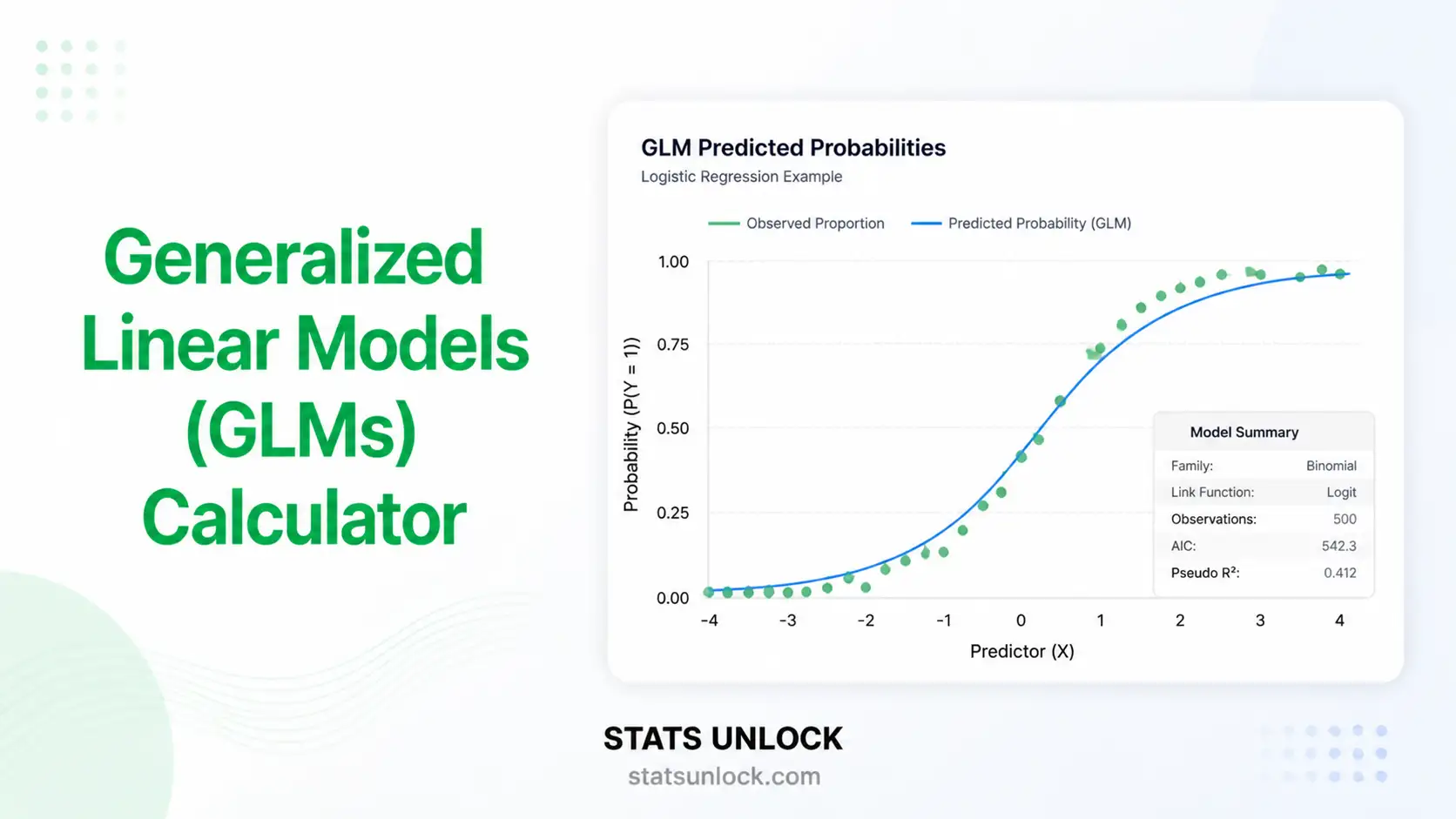
Step 8 — Examine the four plots. Forest plot (effect sizes), observed-vs-predicted (calibration), residuals-vs-fitted (link adequacy), Q-Q plot (distributional fit).
Step 9 — Check assumptions. Pass/Warn/Fail badges flag dispersion, linearity on link scale, and influential outliers.
Step 10 — Export. Download Doc (.txt) for raw output, Download PDF for a formatted report.

9 · Frequently Asked Questions

Q1. What is a Generalized Linear Model (GLM) and when should I use it?

A GLM extends linear regression to outcomes that are not normally distributed — binary, count, proportion, or skewed positive data — by combining a linear predictor with a link function and an exponential-family distribution. Use a GLM when your response variable is binary (logistic), a count (Poisson or Negative Binomial), a positive skewed continuous value (Gamma), or otherwise non-normal.

Q2. What is the difference between linear regression and a GLM?

Linear regression assumes a normally distributed continuous outcome with constant variance. A GLM relaxes both: it allows any distribution from the exponential family (Binomial, Poisson, Gamma, Gaussian, etc.) and uses a link function (logit, log, identity, inverse) to relate the linear predictor η = Xβ to the mean μ of the response.

Q3. How do I interpret GLM coefficients?

GLM coefficients are on the link scale and must be exponentiated for interpretation. For logistic regression, exp(β) is an odds ratio. For Poisson and Negative Binomial (log link), exp(β) is an incidence rate ratio (IRR). For Gamma with log link, exp(β) is a multiplicative effect on the mean. A coefficient of 0 on the link scale corresponds to no effect (exp(0) = 1).

Q4. What is deviance in a GLM and why does it matter?

Deviance is the GLM analogue of the residual sum of squares: D = 2(ℓ_saturated − ℓ_model). The null deviance is the deviance of the intercept-only model; the residual deviance is the deviance of your fitted model. The drop from null to residual deviance, divided by null deviance, gives McFadden's pseudo-R². Smaller residual deviance is better.

Q5. How do I choose between AIC and BIC for GLM model comparison?

Both penalize complexity. AIC = −2ℓ + 2p; BIC = −2ℓ + p·ln(n). BIC penalizes more strongly for large n and tends to favour simpler models. Use AIC for prediction-focused models, BIC when you want to identify the "true" parsimonious structure. Differences greater than 2 are meaningful; greater than 10 is strong evidence.

Q6. What is overdispersion and how do I fix it?

Overdispersion occurs when the observed variance exceeds the variance assumed by the model — most commonly when Poisson regression shows a dispersion ratio (Pearson χ²/residual df) above 1.5. Switch to Negative Binomial regression, which adds a dispersion parameter k, or use quasi-Poisson with an inflated variance. Failing to address overdispersion produces standard errors that are too small and p-values that are too small.

Q7. Which link function should I use?

Use the canonical link for each family unless you have a reason otherwise: logit for Binomial, log for Poisson and Negative Binomial, inverse or log for Gamma, identity for Gaussian. Probit (Φ⁻¹) is an alternative binary link common in econometrics and psychometrics. Complementary log-log is used in discrete-time hazard and survival models.

Q8. How large a sample size does a GLM need?

A common rule is at least 10 events per predictor (EPV) for logistic regression — for example, 50 disease cases support up to 5 predictors. For Poisson and Gamma, aim for 10–20 observations per parameter. With rare events (≤30 cases), use Firth's penalised likelihood to reduce small-sample bias.

Q9. How do I check GLM assumptions?

Check: (1) correct link function via residuals-vs-fitted plot — random scatter is good; (2) absence of overdispersion via the dispersion ratio; (3) independence of observations; (4) linearity on the link scale (for continuous predictors); (5) absence of influential outliers via Cook's distance. The four diagnostic plots in this tool cover the main visual checks.

Q10. Can I use this calculator's output in published research?

This tool is designed for teaching, exploratory analysis, and fast prototyping. For peer-reviewed publication, validate results in R (glm(), MASS::glm.nb()), Python (statsmodels.api.GLM), or SPSS, and report: family, link function, coefficient table with 95% CI, exponentiated effects, AIC/BIC, null and residual deviance, dispersion, and sample size.

10 · References

The following peer-reviewed references support the methods used in this Generalized Linear Models calculator, including logistic regression, Poisson regression, Gamma regression, and Negative Binomial regression. APA 7th edition, with DOIs and verified URLs where available.

Nelder, J. A., & Wedderburn, R. W. M. (1972). Generalized linear models. Journal of the Royal Statistical Society. Series A (General), 135(3), 370–384. https://doi.org/10.2307/2344614
McCullagh, P., & Nelder, J. A. (1989). Generalized Linear Models (2nd ed.). Chapman & Hall/CRC. https://doi.org/10.1201/9780203753736
Agresti, A. (2015). Foundations of Linear and Generalized Linear Models. Wiley. https://www.wiley.com/en-us/Foundations+of+Linear+and+Generalized+Linear+Models
Hosmer, D. W., Lemeshow, S., & Sturdivant, R. X. (2013). Applied Logistic Regression (3rd ed.). Wiley. https://doi.org/10.1002/9781118548387
Cameron, A. C., & Trivedi, P. K. (2013). Regression Analysis of Count Data (2nd ed.). Cambridge University Press. https://doi.org/10.1017/CBO9781139013567
Zuur, A. F., Ieno, E. N., Walker, N. J., Saveliev, A. A., & Smith, G. M. (2009). Mixed Effects Models and Extensions in Ecology with R. Springer. https://doi.org/10.1007/978-0-387-87458-6
Akaike, H. (1974). A new look at the statistical model identification. IEEE Transactions on Automatic Control, 19(6), 716–723. https://doi.org/10.1109/TAC.1974.1100705
Schwarz, G. (1978). Estimating the dimension of a model. The Annals of Statistics, 6(2), 461–464. https://doi.org/10.1214/aos/1176344136
Firth, D. (1993). Bias reduction of maximum likelihood estimates. Biometrika, 80(1), 27–38. https://doi.org/10.1093/biomet/80.1.27
Hilbe, J. M. (2011). Negative Binomial Regression (2nd ed.). Cambridge University Press. https://doi.org/10.1017/CBO9780511973420
Dunn, P. K., & Smyth, G. K. (2018). Generalized Linear Models with Examples in R. Springer. https://doi.org/10.1007/978-1-4419-0118-7
Faraway, J. J. (2016). Extending the Linear Model with R (2nd ed.). CRC Press. https://doi.org/10.1201/9781315382722
Bolker, B. M., Brooks, M. E., Clark, C. J., Geange, S. W., Poulsen, J. R., Stevens, M. H. H., & White, J. S. S. (2009). Generalized linear mixed models: a practical guide for ecology and evolution. Trends in Ecology & Evolution, 24(3), 127–135. https://doi.org/10.1016/j.tree.2008.10.008
R Core Team. (2024). R: A language and environment for statistical computing. R Foundation for Statistical Computing. https://www.R-project.org/
StatsUnlock. (2025). Generalized Linear Models (GLMs) Calculator. Retrieved from https://statsunlock.com/tools/generalized-linear-models-calculator