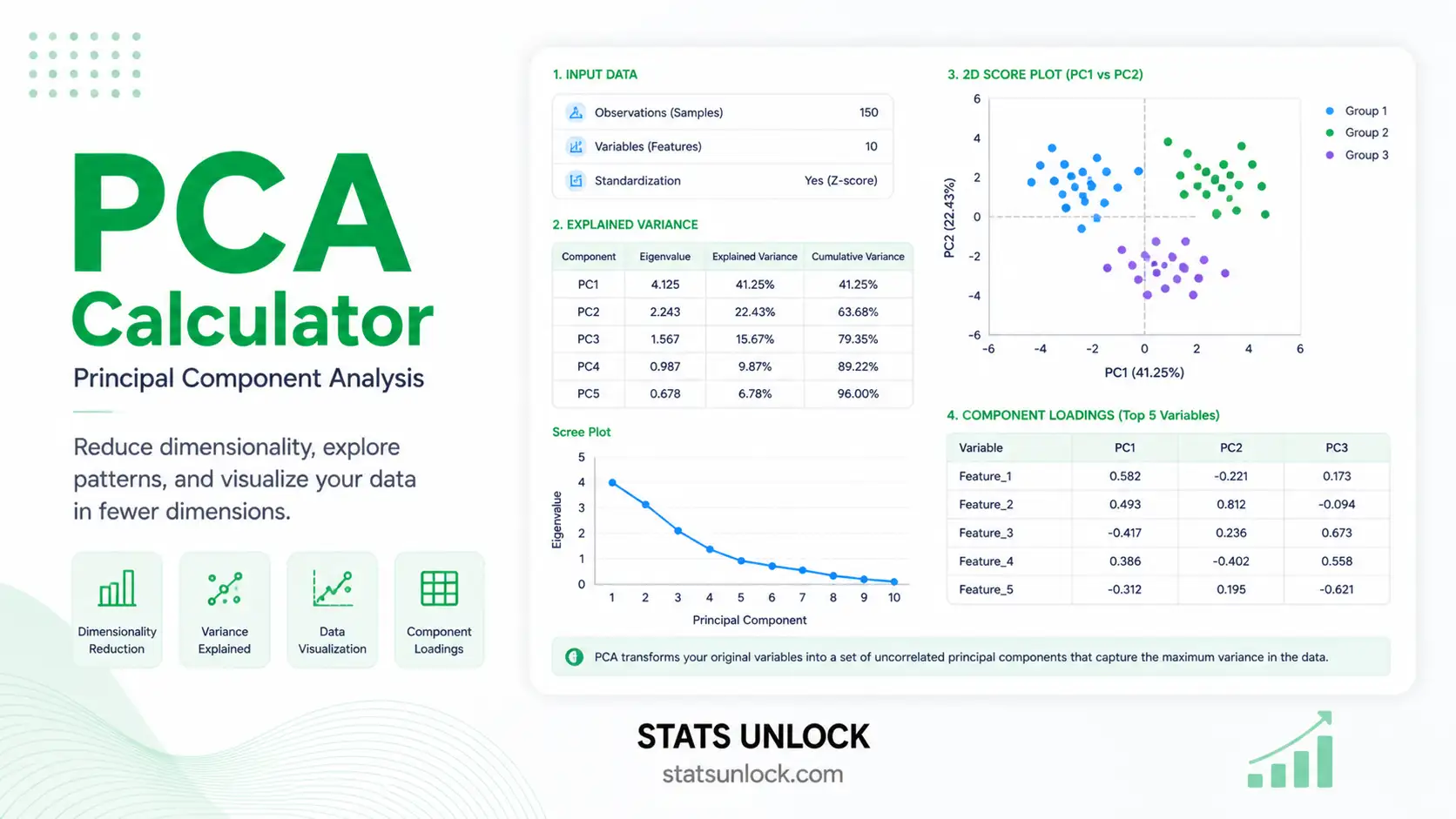
PCA — Principal Component Analysis
Free online Principal Component Analysis calculator: scree plot, biplot, eigenvalues, variance explained, loadings, and component scores — for research, education, and exploratory data analysis.
📥 Data Input
Enter values one per cell. Add rows for more observations; each column is one variable.
🧠 Plain-Language Interpretation & Reporting
Interpretation Results
▶ Run the analysis above to see a detailed interpretation of your PCA results — including what each component represents, how much information is preserved, the loading structure, and what the analysis can and cannot tell you.
How to Write Your Results in Research
Five ready-to-use reporting templates, auto-filled after you run the analysis. Click 📋 Copy to send the example to your clipboard.
🎯 Conclusion
Principal Component Analysis is one of the most widely used multivariate techniques in modern statistics, ecology, psychology, finance, genomics, and machine learning. Its purpose is straightforward but powerful — it takes a set of correlated variables and rebuilds them as a smaller set of uncorrelated principal components, ordered so that the first component captures the maximum possible variance, the second captures the next most, and so on. The result is a compressed yet faithful representation of your data, with the noise stripped away from the dominant signal.
This calculator computes PCA from first principles in your browser. It standardizes the variables (or uses raw covariance, depending on your selection), builds the correlation or covariance matrix, runs an iterative eigen-decomposition (Jacobi rotations), and then derives eigenvalues, eigenvectors (loadings), component scores, % variance explained, and cumulative variance. Four colorful visualizations — a scree plot, a cumulative variance curve, a biplot, and a loadings bar chart — allow you to see the structure at a glance.
Key take-aways for your research:
- PC1 is always the most important component by construction; it is the linear combination of variables that maximally separates observations along one axis.
- The number of components to retain is a judgement call — combine the Kaiser rule (eigenvalue > 1), the scree-plot elbow, and the cumulative-variance threshold (usually 70–90%).
- Loadings tell you the meaning of each component — variables with large absolute loadings define what the component represents.
- Scores are the position of each observation on each component — use them as inputs to clustering, regression, or visualisation.
- PCA is a descriptive tool. It does not test a hypothesis, prove causality, or guarantee that the components are interpretable. It is exploratory by nature.
- Always standardize your data when variables are measured in different units, otherwise the variable with the largest raw variance will dominate the first component artificially.
Used carefully, PCA is one of the most rewarding analyses you can run on a multivariate dataset. It reveals which variables move together, which observations stand apart, and how much of your data's complexity can be summarised in just a few dimensions. Combined with the interpretation templates above, the results from this tool can flow directly into a thesis Methods section, a peer-reviewed Results paragraph, a conference abstract, a policy brief, or a pre-registration plan — without manual reformatting. For confirmatory analysis, follow up with Factor Analysis (EFA / CFA), Cluster Analysis, or LDA depending on whether your goal is latent-structure modelling, grouping, or classification.
📐 Technical Notes & Formulas
📌 Formulas Used
1. Standardization (z-score)
zij = (xij − x̄j) / sj

Where:
  zij = standardized value of observation i on variable j
  x̄j  = sample mean of variable j
  sj   = sample standard deviation of variable j (n-1 divisor)
2. Correlation (or Covariance) Matrix
R = (1 / (n−1)) · ZT · Z   (correlation, after z-scoring)
S = (1 / (n−1)) · XcT · Xc   (covariance, raw or centered)

Where:
  R   = p × p correlation matrix
  S   = p × p covariance matrix
  Z   = n × p standardized data matrix
  Xc  = n × p centered raw data matrix
  n   = number of observations
  p   = number of variables
3. Eigen-Decomposition
R · vk = λk · vk

Where:
  λk  = k-th eigenvalue (variance captured by PC k)
  vk  = k-th eigenvector (column of loadings for PC k)
  Sum of eigenvalues = total variance = p (when using R)
4. Variance Explained
VarExpk      = λk / Σλ
CumVark      = Σi=1..k VarExpi
Total variance   = Σλk = p (correlation) or = trace(S) (covariance)
5. Component Scores
F = Z · V

Where:
  F   = n × p matrix of component scores
  Z   = n × p standardized data
  V   = p × p matrix of eigenvectors (columns sorted by descending λ)
6. Loadings (correlation between variable and component)
Ljk = vjk · √λk

Where:
  Ljk = loading of variable j on component k
  vjk = j-th element of the k-th eigenvector
  √λk = standard deviation of PC k
7. Communality & Kaiser Rule
hj2 = Σk retained Ljk2      (communality of variable j)
Retain PC k if λk > 1   (Kaiser–Guttman rule, only for correlation PCA)
🛠️ Technical Notes
Algorithm. The calculator performs eigen-decomposition using the classical Jacobi rotation method, which is exact for symmetric matrices and stable for the small-to-medium-p problems that PCA is normally applied to. For very large datasets (p > 100), production tools should use SVD-based PCA from R, Python, or SPSS for numerical efficiency.
Standardization. When variables are measured in different units (cm vs kg vs $), always standardize before computing PCA — otherwise the eigen-decomposition will be dominated by whichever variable has the largest raw scale. Standardization is equivalent to running PCA on the correlation matrix.
Sign convention. Eigenvectors are unique only up to a sign flip. Two software packages may report loadings with opposite signs — this is mathematically equivalent and does not change the interpretation, only the orientation of the axis.
Sample size. A common rule of thumb is at least 5–10 observations per variable, with a minimum total n of 100–300 for stable loadings. Smaller samples are still usable for exploratory work but loadings become unstable.
✅ When to Use Principal Component Analysis
📌 Decision checklist + real-world examples
PCA is appropriate when:
- ✅ You have multiple continuous variables measured on the same observations
- ✅ The variables are at least moderately correlated (otherwise PCA cannot reduce dimensions)
- ✅ Your goal is data exploration, dimensionality reduction, or visualisation
- ✅ You want to remove multicollinearity before regression
- ✅ You want a small number of uncorrelated features for clustering or downstream modelling
- ❌ Do not use if your variables are categorical → use MCA / FAMD
- ❌ Do not use if you want to test a confirmatory latent-structure hypothesis → use Confirmatory Factor Analysis (CFA)
- ❌ Do not use raw (unscaled) data when units differ → standardize first
Real-world examples
- Ecology / Wildlife. Reducing 8 habitat variables (canopy cover, leaf litter, soil moisture, temperature, etc.) to 2–3 components representing "habitat moistness" and "vegetation density".
- Psychology. Compressing a 20-item personality scale into 3–5 latent dimensions for downstream regression on outcomes.
- Finance. Building a "market factor" from 50 stock returns — PC1 typically explains the broad market direction.
- Genomics. Visualising thousands of gene-expression measurements for hundreds of samples in a 2-D PC1–PC2 space to detect batch effects and clustering by tissue or disease.
📖 How to Use This Tool
📌 Step-by-step guide (worked example)
Step 1 — Enter Your Data
Pick one of the three tabs: Paste / Type (default — comma-separated values), Upload CSV / Excel, or Manual Entry. Each variable is one block. Group names (variable names) are editable.
Step 2 — Choose a Sample Dataset
The top dropdown loads one of five teaching datasets (Iris, Wine, Habitat, Finance, Psychology). They demonstrate what good PCA-ready data looks like.
Step 3 — Configure Preprocessing
Choose Standardize (z-score) for variables on different scales (recommended), Center only when variables are on the same scale, or Raw when you specifically want a covariance-matrix PCA.
Step 4 — Run the Analysis
Click ▶ Run PCA Analysis. The Results card unfolds with summary cards, full tables, four charts, and dynamic interpretation.
Step 5 — Read the Summary Cards
The four cards show: number of variables, number of observations, % variance in PC1, and cumulative variance explained by the first two components.
Step 6 — Read the Full Tables
The eigenvalue table shows λ, % variance, and cumulative %. The loadings table shows how each variable contributes to each component.
Step 7 — Examine the Four Visualizations
Scree plot — find the elbow. Cumulative variance — find the 70/80/90% threshold. Biplot — interpret PC1 and PC2 in terms of variables and observations. Loadings bar chart — see at a glance which variables drive each component.
Step 8 — Check Assumptions
Verify your variables are continuous, that they are at least moderately correlated, and that you have enough sample size. The interpretation block flags small-n warnings automatically.
Step 9 — Read the Interpretation
Use the dynamically generated interpretation paragraphs verbatim in your thesis or report. Then pick the best of the five reporting templates (APA, dissertation, plain-language, abstract, pre-registration) and click 📋 Copy.
Step 10 — Export Your Results
Use 📋 Download Doc for a plain-text report, or 🖨️ Download PDF to print/save a publication-ready PDF.
❓ Frequently Asked Questions
Q1. What is Principal Component Analysis (PCA) and when should I use it?
PCA is an unsupervised, descriptive multivariate technique that transforms a set of correlated continuous variables into a smaller set of uncorrelated principal components ordered by the variance they capture. Use it when you have many correlated variables and want to reduce dimensions, visualise multivariate structure, remove multicollinearity, or compress data while keeping most of the variance — common in ecology, psychometrics, genomics, finance, and image analysis.
Q2. PCA does not produce a p-value — how do I assess "significance"?
PCA is descriptive, not inferential, so there is no traditional p-value. "Significance" here is judged by how much variance each component explains and whether that variance is more than what would be expected from random data. Common tools include the Kaiser rule (λ > 1), parallel analysis (Horn, 1965), the scree-plot elbow, and a cumulative-variance threshold of 70 to 90 percent.
Q3. Statistical vs practical importance — what counts as a meaningful component?
A component is "important" when it explains a substantial share of the total variance and has a clear, interpretable loading pattern. A component that captures 1 percent of variance is rarely useful even if its eigenvalue is technically positive. As a rule of thumb, only components that explain at least 5–10 percent and that load substantively on multiple original variables are worth interpreting.
Q4. What are loadings and how do I interpret them?
Loadings are the correlation between each original variable and each principal component (after multiplying eigenvectors by √λ). Absolute values close to 1 indicate strong contribution, values close to 0 indicate weak contribution. By convention, loadings with |L| ≥ 0.30 are usually considered meaningful, |L| ≥ 0.50 are strong, and |L| ≥ 0.70 are very strong. Their sign indicates the direction of the relationship along the component.
Q5. What assumptions does PCA make, and what if my data violate them?
PCA assumes (1) continuous numeric variables, (2) at least moderate inter-correlation, (3) approximate linearity of relationships, and (4) sufficient sample size. If your variables are categorical, switch to MCA or FAMD. If correlations are near zero, PCA cannot reduce dimensions — your data are already nearly orthogonal. If relationships are clearly non-linear, consider Kernel PCA, t-SNE, or UMAP. The Kaiser–Meyer–Olkin (KMO) statistic and Bartlett's test of sphericity are commonly reported as factorability checks.
Q6. How large a sample do I need for PCA to be reliable?
Common rules of thumb are at least 5–10 observations per variable and a total n of 100–300. Comrey and Lee (1992) classify n = 100 as poor, 200 as fair, 300 as good, 500 as very good, and 1000+ as excellent. For exploratory teaching examples, smaller samples (n = 20–50) are acceptable but loadings will be unstable.
Q7. Should I rotate the components after PCA?
Rotation (Varimax, Quartimax, Promax) is more common in Exploratory Factor Analysis than in PCA. If you keep more than one component and want them to be more interpretable — each variable loading high on one component and low on the others — Varimax (orthogonal) rotation can help. Note that rotated PCA loses the property that PC1 captures the maximum variance.
Q8. How do I report PCA results in APA 7th edition format?
Report sample size, whether data were standardized, the rotation method (if any), the number of components retained and the rule used (Kaiser, scree, parallel analysis), the eigenvalues and percent variance explained per component, the cumulative variance, and the loading matrix. Bartlett's test and KMO should also be reported when used. See the five auto-filled reporting templates above for ready-to-use wording.
Q9. Can I use this calculator for my published research or university assignment?
Yes for educational and exploratory work. For peer-reviewed publications, we recommend re-running the analysis in established software (R prcomp/princomp, Python scikit-learn, SPSS, SAS PROC FACTOR) and citing both. Citation: STATS UNLOCK. (2026). PCA — Principal Component Analysis calculator. Retrieved from https://statsunlock.com.
Q10. PC1 explains very little variance — what does that mean?
It means the variables are nearly uncorrelated, so PCA cannot meaningfully compress them — each variable already carries roughly independent information. In that case, dimensionality reduction will not help; treat each variable on its own or use a non-linear method (UMAP, t-SNE) to look for structure that linear PCA cannot capture.
📚 References
📌 References (APA 7th edition, with links)
The following references support the statistical methods used in this Principal Component Analysis tool, covering eigen-decomposition, variance explained, component loadings, and best practices in multivariate data analysis.
- Pearson, K. (1901). On lines and planes of closest fit to systems of points in space. Philosophical Magazine, 2(11), 559–572. https://doi.org/10.1080/14786440109462720
- Hotelling, H. (1933). Analysis of a complex of statistical variables into principal components. Journal of Educational Psychology, 24(6), 417–441. https://doi.org/10.1037/h0071325
- Jolliffe, I. T. (2002). Principal Component Analysis (2nd ed.). Springer. https://doi.org/10.1007/b98835
- Jolliffe, I. T., & Cadima, J. (2016). Principal component analysis: A review and recent developments. Philosophical Transactions of the Royal Society A, 374(2065), 20150202. https://doi.org/10.1098/rsta.2015.0202
- Kaiser, H. F. (1960). The application of electronic computers to factor analysis. Educational and Psychological Measurement, 20(1), 141–151. https://doi.org/10.1177/001316446002000116
- Cattell, R. B. (1966). The scree test for the number of factors. Multivariate Behavioral Research, 1(2), 245–276. https://doi.org/10.1207/s15327906mbr0102_10
- Horn, J. L. (1965). A rationale and test for the number of factors in factor analysis. Psychometrika, 30(2), 179–185. https://doi.org/10.1007/BF02289447
- Abdi, H., & Williams, L. J. (2010). Principal component analysis. Wiley Interdisciplinary Reviews: Computational Statistics, 2(4), 433–459. https://doi.org/10.1002/wics.101
- Tabachnick, B. G., & Fidell, L. S. (2019). Using Multivariate Statistics (7th ed.). Pearson.
- Comrey, A. L., & Lee, H. B. (1992). A First Course in Factor Analysis (2nd ed.). Lawrence Erlbaum Associates.
- Field, A. (2018). Discovering Statistics Using IBM SPSS Statistics (5th ed.). SAGE Publications.
- American Psychological Association. (2020). Publication Manual of the American Psychological Association (7th ed.). APA. https://doi.org/10.1037/0000165-000
- R Core Team. (2024). R: A language and environment for statistical computing. R Foundation for Statistical Computing. https://www.R-project.org/
- Pedregosa, F., et al. (2011). Scikit-learn: Machine learning in Python. Journal of Machine Learning Research, 12, 2825–2830. https://jmlr.org/papers/v12/pedregosa11a.html
- NIST/SEMATECH. (2013). e-Handbook of statistical methods — Principal Components Analysis. National Institute of Standards and Technology. https://www.itl.nist.gov/div898/handbook/pmc/section5/pmc55.htm


