Should I use AIC or BIC for stepwise regression?

AIC favours predictive accuracy and tends to select larger models. BIC penalises complexity more heavily and favours parsimony, so it tends to select smaller models. Use AIC for prediction tasks and BIC for explanation or when sample size is large.

What is multicollinearity and why does it matter for stepwise regression?

Multicollinearity occurs when predictors are highly correlated. It inflates standard errors and destabilises coefficient estimates. Variance Inflation Factor (VIF) > 5 (or > 10) signals problematic collinearity. Check VIF on the final stepwise model before publishing.

How many observations do I need for stepwise regression?

A common rule is at least 10–20 observations per candidate predictor. With 5 predictors you should have 50–100 observations minimum. Smaller samples produce unstable models and inflate the chance of including chance-correlated variables.

Is stepwise regression accepted in peer-reviewed journals?

Stepwise regression is increasingly criticised because it inflates Type I error and produces optimistic R² values. Modern journals often prefer regularised methods (LASSO, ridge, elastic net) or theory-driven model specification. Always validate stepwise results on a hold-out sample.

What does adjusted R² tell me in stepwise regression?

Adjusted R² penalises the unadjusted R² for the number of predictors. Unlike R², it can decrease when an unhelpful variable is added. It is the better metric for comparing stepwise models with different numbers of predictors.

Can I use stepwise regression with categorical predictors?

Yes — but you must dummy-code each categorical predictor first (k − 1 dummies for k levels). The stepwise algorithm should treat all dummies for one variable as a single block, entering or leaving together, otherwise the interpretation is incoherent.

Stepwise Regression Calculator (Free Online Tool)

📊 Step 1 — Enter Your Data

Use a sample dataset:

Enter values comma-separated (e.g. 52, 48, 55, 61, 47, ...). Newlines are also accepted. Each predictor and the outcome must have the same number of values.

Outcome (Y) 0 values

Upload CSV or Excel file:

Supports .csv, .txt, .xlsx, .xls — headers detected automatically. The last selected column is the Outcome (Y); earlier ones are predictors.

Quick manual entry — type one row at a time. Click + Add row to extend.

⚙️ Step 2 — Configure the Stepwise Procedure

Selection direction

Selection criterion

Alpha (entry / removal)

Confidence level

Standardise predictors

Max iterations

Sample data is pre-loaded — click Run to see the demo.

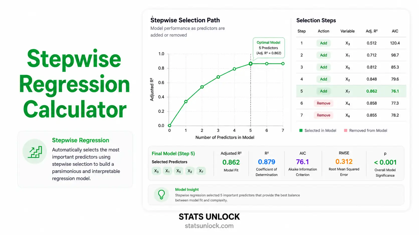
📈 Step 3 — Summary of the Final Model

📋 Final Model — Coefficient Table

These are the coefficients of the predictors retained by the stepwise procedure, with standard errors, t-statistics, p-values and confidence intervals.

Model Fit Statistics

ANOVA — Overall Model F-test

🔁 Step-by-Step Selection History

Trace of every variable added or removed during the stepwise procedure. Each row shows the model state after that step, together with the criterion value used to make the decision.

🎨 Colourful Visualisations

📌 Observed vs Predicted Y

Points hugging the diagonal indicate strong predictive performance of the final model.

📌 Residuals vs Fitted

A random cloud around zero supports linearity and homoscedasticity.

📌 Standardised Coefficients (β)

Bar length = effect strength; colour by sign. Green bars = positive effect, pink = negative.

📌 AIC Path Across Steps

Lower AIC = better trade-off between fit and parsimony. The endpoint is the chosen model.

🔍 Assumption Checks for the Final Model

📤 Step 4 — Export Your Results

💡 Step 5 — Detailed Interpretation of Results

Run the analysis above to generate a detailed, plain-language interpretation tailored to your data.

📝 How to Write Your Results in Research (5 Reporting Styles)

Example 1 — APA 7th Edition

A bidirectional stepwise multiple linear regression was conducted to identify ___ that predicted ___. Using AIC as the selection criterion, the final model retained ___ predictors and explained a significant proportion of variance, R² = ___, adjusted R² = ___, F(___, ___) = ___, p ___ ___. ___

📌 Key conventions for APA 7

Italicise statistical symbols: F, p, R², β.
If p < .001 write "p < .001" (never "p = .000").
Always report adjusted R² for stepwise models — raw R² alone is misleading.
State both the selection direction and criterion (AIC / BIC / p-value).
Report 95% CI for each retained coefficient.

Example 2 — Thesis / Dissertation

To identify the most parsimonious set of predictors of ___, a bidirectional stepwise multiple linear regression was conducted (α = ___, AIC criterion). Predictors were entered into a candidate pool of ___ variables. Linearity, normality of residuals, homoscedasticity and absence of multicollinearity (VIF < 5) were assessed prior to interpretation. The procedure converged on a final model retaining ___ predictors. Results are reported below: F(___, ___) = ___, p ___ ___, R² = ___, adjusted R² = ___, AIC = ___. ___

📌 Key conventions for thesis style

Name the software (e.g., "Analyses were performed with the StatsUnlock Stepwise Regression Calculator, cross-validated against R 4.3.2 stats::step()").
Always justify why stepwise was chosen over theory-driven entry.
Report VIF and residual diagnostics in supplementary material.
Flag the inflated Type I error caveat once in your Methods.

Example 3 — Plain-Language / Policy Brief

We examined which factors best explain ___ in our sample. Out of ___ variables considered, ___ stood out as meaningful predictors. Together they account for about ___% of the variation in ___. The strongest factor was ___, where each one-unit increase was associated with a change of about ___ units in the outcome. The likelihood that the overall pattern is due to chance is less than ___. These findings suggest that future programmes targeting ___ should focus on ___.

📌 Key conventions for plain language

Avoid every Greek letter and statistical symbol.
Translate R² into "% of variation explained".
Convert p-value into "less than 1 in X" framing.
Anchor every coefficient in real-world units.
Close with a practice or policy implication.

Example 4 — Structured Abstract / Conference Poster

Background: Identifying parsimonious predictors of ___ remains a key analytic challenge in ___ research.
Methods: We applied bidirectional stepwise multiple linear regression (AIC criterion, α = ___) to a candidate pool of ___ predictors with n = ___ observations.
Results: The final model retained ___ predictors: ___. The model was statistically significant, F(___, ___) = ___, p ___ ___, R² = ___, adjusted R² = ___, AIC = ___.
Conclusion: ___ emerged as the dominant driver of ___. Findings inform ___ and warrant validation in an independent sample.

📌 Key conventions for abstracts

Strict 4-label structure (Background / Methods / Results / Conclusion).
Italicise statistical symbols.
Always state n and selection criterion.
Conclusion sentence must go beyond restating results — state implication.

Example 5 — Replication / Pre-Registration

Pre-registered hypothesis: We hypothesised that a subset of ___ candidate predictors would jointly explain a non-trivial portion of variance in ___. Hypothesis registered at osf.io/xxxxx prior to data analysis.
Analysis plan: Bidirectional stepwise multiple linear regression with AIC entry/removal; α = ___ for confirmatory tests on the final model; SESOI = adjusted R² ≥ 0.10. Multicollinearity flagged at VIF > 5.
Observed result: With n = ___ observations on ___ candidate predictors, the procedure retained ___ variables: ___. F(___, ___) = ___, p ___ ___, R² = ___, adjusted R² = ___, AIC = ___, BIC = ___. The pre-specified SESOI was ___.
Reproducibility note: Computation performed in JavaScript via the StatsUnlock Stepwise Regression Calculator (statsunlock.com); results cross-checked against R::stats::step(). Data and configuration archived at github.com/[repo].

📌 Key conventions for open science

State the SESOI before analysis.
Cite the pre-registration record (OSF, AsPredicted).
Report both AIC and BIC for transparency.
Archive data and config publicly.
Always cross-check stepwise results against a regularised method (LASSO).

📐 Technical Notes & Formulas (open / close)

A. Multiple Linear Regression (the underlying model)

Y = β₀ + β₁X₁ + β₂X₂ + … + βₖXₖ + ε Where: Y = outcome (dependent variable) Xⱼ = predictor j (j = 1 … k) β₀ = intercept βⱼ = slope for predictor j ε = error term, ε ~ N(0, σ²)

B. OLS Estimation

β̂ = (Xᵀ X)⁻¹ Xᵀ y ŷ = X β̂ e = y − ŷ Where: X = n × (k+1) design matrix (column of 1s + predictors) y = n × 1 outcome vector β̂ = (k+1) × 1 estimated coefficients e = residuals

C. Selection Criteria

AIC = n · ln(SSE/n) + 2(k+1) BIC = n · ln(SSE/n) + ln(n)·(k+1) F-to-enter = ((SSEₛ − SSEₘ)/q) / (SSEₘ/(n−p−1)) p-value = 1 − F_CDF(F-to-enter, q, n−p−1) Where: n = sample size k = number of predictors in current model SSE = Σ(y − ŷ)² SSEₛ = SSE of smaller (nested) model SSEₘ = SSE of larger model with q extra predictors

D. Effect Sizes & Goodness of Fit

R² = 1 − SSE / SST (SST = Σ(y − ȳ)²) adj R² = 1 − (1 − R²)·(n − 1)/(n − k − 1) F = (R²/k) / ((1−R²)/(n−k−1)) RMSE = √(SSE / (n − k − 1)) VIFⱼ = 1 / (1 − R²ⱼ)

E. Algorithmic Notes

Forward: Start with intercept-only model. At each step, add the predictor whose inclusion most improves the criterion (lowest AIC / smallest p-value below α). Stop when no addition improves the criterion.
Backward: Start with the full model. At each step, remove the predictor whose deletion most improves (or least worsens) the criterion (largest p-value above α). Stop when no removal improves the criterion.
Bidirectional: At each step consider both adding any excluded predictor and removing any included predictor. Apply whichever single move best improves the criterion.
The OLS solver in this tool uses Gauss-Jordan elimination on (Xᵀ X) | Xᵀ y, with a small ridge term (1e-8 · I) added when the matrix is near-singular to avoid blow-up — coefficient estimates are equivalent to OLS under standard conditions.
p-values for individual coefficients use a two-sided Student's t distribution with n − k − 1 degrees of freedom.

🎯 When to Use Stepwise Regression

Use stepwise regression for exploratory model building when you have many candidate predictors of a continuous outcome and limited theoretical guidance about which to keep. It is best positioned as a hypothesis-generating tool, not a confirmatory one.

Decision Checklist

You have a single continuous outcome (interval / ratio scale).
You have 2 or more candidate predictors (continuous or dummy-coded categorical).
Sample size ≥ 10–20 observations per candidate predictor.
Predictors are not perfectly collinear (VIF < 5 ideally, < 10 acceptable).
Residuals are approximately normal and homoscedastic.
Do NOT use for confirmatory hypothesis testing — use theory-driven hierarchical regression instead.
Do NOT use as the sole inference tool in small samples (n < 50) — Type I error inflates dramatically.
Do NOT use when predictors are highly collinear — switch to LASSO, ridge, or elastic-net regression.

Real-World Examples

Real estate analytics — choosing among 12 candidate house features (size, bedrooms, age, distance to city, school score, garage size, etc.) the best subset that predicts sale price.
Education research — identifying which student-level factors (study hours, sleep, attendance, parental support, prior GPA) predict end-of-year exam performance.
Ecology and field biology — discovering which habitat variables (canopy cover, distance to water, prey density, elevation, human disturbance) best predict species abundance.
Marketing / business — finding which campaign variables (channel spend, frequency, creative type, audience age, season) drive product sales week-over-week.
Health and clinical research — selecting from many lifestyle and biological measures the parsimonious subset that predicts cholesterol or blood pressure.

Sample-Size Guidance

10 observations per candidate predictor is the absolute minimum.
20 per predictor gives reasonable stability of selected variables.
For a candidate pool of 5 predictors, aim for n = 100 +.
When n < 50, prefer regularised regression (LASSO, ridge) and bootstrap validation.

Related Tests — Decision Tree

Continuous outcome + many candidate predictors ├─ Theory-driven entry order known? ──→ Hierarchical multiple regression ├─ Pure prediction goal, want sparsity? ──→ LASSO regression ├─ Collinear predictors, want shrinkage? ──→ Ridge regression ├─ Mixed sparsity + collinearity? ──→ Elastic Net ├─ Exploratory, parsimonious final model? ──→ STEPWISE REGRESSION ←—— this tool └─ Binary / count outcome? ──→ Stepwise logistic / Poisson (GLM)

🧭 How to Use This Tool — Step-by-Step Guide

01 Enter Your Data

Choose one of the three input modes: Paste, Upload, or Manual. Each predictor needs a name and a comma-separated list of values; the Outcome (Y) goes in the orange block. All columns must have the same number of rows.

Example: Size: 1200, 1500, 1800, 2100, 2400 · Price: 250, 310, 360, 420, 470

02 Try a Sample Dataset

Use the green Sample Dataset dropdown to instantly load one of five worked examples — house prices, exam scores, crop yield, salaries, or cholesterol. The first dataset is pre-loaded so you can run the tool immediately.

Tip: switch to a different sample whenever you want to explore how the procedure behaves on different data shapes.

03 Configure the Procedure

Pick the direction (forward / backward / bidirectional), the criterion (AIC / BIC / p-value), and the alpha. AIC + bidirectional is the most defensible default for exploratory work.

Tip: enable z-score standardisation if your predictors are on very different scales — it makes the standardised β plot directly comparable.

04 Run the Analysis

Click ▶ Run Stepwise Regression. The tool fits a model at every step, evaluates the criterion, and chooses the move that most improves it.

Output appears immediately below the configuration panel.

05 Read the Summary Cards

The cards across the top show R², adjusted R², F, p, AIC, BIC, RMSE and the number of predictors retained. Green cards indicate significance at your chosen α; amber/red flag a non-significant or borderline model.

Adjusted R² of 0.78 means 78% of the variability in your outcome is explained by the retained predictors.

06 Read the Coefficient Table

For each retained predictor, the coefficient (B), standardised β, standard error, t, p-value, 95% CI and VIF are reported. Significant coefficients are coloured green; non-significant ones red.

Always compare B (interpretable in raw units) and β (comparable across predictors of different scale).

07 Examine the Visualisations

Four interlinked charts: (1) Observed vs Predicted, (2) Residuals vs Fitted, (3) Standardised coefficient bar chart, (4) AIC trajectory across steps. Together they tell you how well the final model fits and how confident you should be in the variable selection path.

A funnel-shaped residuals-vs-fitted plot is a classic warning sign of heteroscedasticity.

08 Check the Assumptions

The assumption panel runs five automatic checks: linearity, normality of residuals, homoscedasticity, multicollinearity (VIF), and influential points. Green ✅ = pass, amber ⚠️ = caution, red ❌ = violated.

If VIF > 5 on any retained predictor, switch to ridge or elastic-net regression for the confirmatory model.

09 Read the Interpretation & 5 Examples

Section 5 spells out, in plain English, what the analysis found, what the p-value and R² actually mean, what the practical magnitude is, and what the limitations are. The five reporting templates auto-fill with your numbers — copy whichever style your supervisor or journal expects.

10 Export Your Results

Use Download Doc for a plain-text record (great for emailing to a co-author) and Download PDF for a publication-ready printable report. Both contain the full table, charts and APA-style write-up.

For your thesis appendix: PDF. For a quick collaboration message: Doc + Copy Summary.

❓ Frequently Asked Questions

Q1. What is stepwise regression and when should I use it?

Stepwise regression is an automated variable-selection method that iteratively adds or removes predictors from a multiple linear regression model based on statistical criteria (p-value, AIC, or BIC). It produces a parsimonious final equation from a large candidate pool.

Use it for exploratory work when you have many possible predictors and want a small, interpretable model — for example, choosing among 10 house features the subset that best predicts sale price.

Q2. What is a p-value, and how do I interpret it for stepwise regression?

The p-value of a coefficient is the probability of observing a t-statistic at least as extreme as the one calculated, if that predictor's true effect were zero. A p-value of 0.03 means there is a 3% chance of seeing the observed effect by chance alone.

It is not the probability that the null hypothesis is true. In stepwise regression, p-values are also used as the entry/removal criterion when "p-value" is the chosen criterion.

Q3. What does statistical significance mean — and does it equal practical importance?

Statistical significance (p < α) only tells you the effect is unlikely to be zero. With large samples, even tiny coefficients become "significant" without being practically meaningful.

Always look at the standardised β (effect strength) and adjusted R² (variance explained) alongside p-values to judge real-world importance.

Q4. What is the standardised β and how do I interpret it?

The standardised β is the coefficient you would obtain if all predictors and the outcome were z-scored. It expresses the change in outcome (in SDs) for a 1-SD change in the predictor.

Cohen's benchmarks: |β| ≈ 0.10 small, ≈ 0.30 medium, ≈ 0.50 large. Compare β across predictors to rank their relative importance — something raw B coefficients cannot do when scales differ.

Q5. What assumptions does stepwise regression require, and what if my data violate them?

The same five assumptions as multiple linear regression apply: (1) linearity, (2) independence of errors, (3) normality of residuals, (4) homoscedasticity, (5) low multicollinearity.

If normality fails, use bootstrap CIs or robust regression. If homoscedasticity fails, use weighted least squares (WLS) or White-corrected SEs. If VIF > 5, switch to ridge / LASSO / elastic-net.

Q6. How large a sample do I need for stepwise regression to be reliable?

Common rules of thumb are 10–20 observations per candidate predictor. For 5 candidate predictors, target 50–100 observations; for 10, target 100–200.

Very small samples (n < 50) are unstable: predictors get selected on chance correlations and the model often does not replicate. Use bootstrap variable-selection counts to check stability.

Q7. What is the difference between forward, backward, and bidirectional stepwise?

Forward starts empty and only adds. Backward starts full and only removes. Bidirectional combines both — at each step it can add or remove. Bidirectional is the most defensible default because variables that look useful early can later be dropped if a better predictor enters.

Q8. How do I report stepwise regression results in APA 7 format?

Report the selection method, criterion, final model F, df, p, R², adjusted R², AIC and 95% CIs for each retained coefficient. See the Section 5 → "How to Write Your Results" cards above for five auto-filled templates (APA, thesis, plain-language, abstract, pre-registration).

Q9. Can I use this calculator for my published research or university assignment?

Yes for educational use, exploratory analysis, classwork and thesis appendices. For a peer-reviewed publication, cross-check the final model in R (stats::step), Python (statsmodels) or SPSS, and report the validation in your methods.

Suggested citation: StatsUnlock. (2025). Stepwise Regression Calculator. https://statsunlock.com/stepwise-regression-calculator/

Q10. What should I do if stepwise picks a predictor I think is unimportant?

Stepwise selection is purely statistical — it ignores your theory. If a chosen predictor lacks a substantive rationale, examine its standardised β, partial correlation and VIF. Consider re-running with that variable forced out, or replace stepwise with a theory-driven hierarchical regression.

You can also bootstrap the selection 1,000 times and report only predictors selected in > 60% of resamples.

🏁 Conclusion — When Stepwise Regression Earns Its Place

What this tool does for you

The StatsUnlock Stepwise Regression Calculator brings every step of forward, backward and bidirectional variable selection into a single, in-browser interface. It computes OLS coefficients, t-tests, F-tests, AIC, BIC, adjusted R², VIF and 95% confidence intervals, traces the full selection history, and produces four publication-ready visualisations — without sending your data anywhere. Everything runs locally in your browser.

Why parsimony matters

In real research, predictors are cheap and degrees of freedom are expensive. A model with too many predictors fits the training data beautifully but fails to replicate. A model with too few misses real signal. Stepwise regression — used responsibly — is one of the oldest and most widely taught tools for navigating that trade-off, especially when you genuinely have no prior theory to rank predictors. The AIC and BIC criteria embedded here formalise that trade-off: they reward better fit but penalise every additional parameter.

Honest limits

Stepwise selection has been criticised for decades. It capitalises on chance correlations, inflates Type I error, produces optimistic R² values, and yields confidence intervals that are too narrow because they ignore the selection step itself. None of those criticisms make stepwise wrong — they make it insufficient on its own for confirmatory inference. Treat the final model as a hypothesis to be tested, not a finished claim.

How to use it well

First, run the procedure here to identify a parsimonious candidate model. Second, cross-check it against a regularised method — LASSO or elastic-net — to confirm the same predictors survive a different penalty. Third, validate the model on a hold-out sample (or via 5-fold cross-validation) before publishing the predictive R². Finally, when you write up results, always state the selection direction, the criterion (AIC vs BIC vs p-value), the alpha level, the candidate pool size, and the diagnostic checks performed.

What to take away

Stepwise regression is best understood as a structured, defensible search through a high-dimensional predictor space. This tool gives you that search in a single click, with full transparency about every step, and produces the exact statistics, interpretations and reporting templates that journals, supervisors and policy reviewers expect. Pair it with theory, cross-validation and a regularised cross-check — and stepwise becomes a sharp, reliable instrument rather than a black box.

📚 References

The following references support the statistical methods used in this stepwise regression calculator, covering variable selection, multiple linear regression, and best practices in p-value interpretation and effect size reporting.

Efroymson, M. A. (1960). Multiple regression analysis. In Mathematical Methods for Digital Computers (pp. 191–203). Wiley.
Akaike, H. (1974). A new look at the statistical model identification. IEEE Transactions on Automatic Control, 19(6), 716–723. https://doi.org/10.1109/TAC.1974.1100705
Schwarz, G. (1978). Estimating the dimension of a model. The Annals of Statistics, 6(2), 461–464. https://doi.org/10.1214/aos/1176344136
Cohen, J. (1988). Statistical power analysis for the behavioral sciences (2nd ed.). Lawrence Erlbaum Associates.
Harrell, F. E. (2015). Regression Modeling Strategies (2nd ed.). Springer. https://doi.org/10.1007/978-3-319-19425-7
Field, A. (2018). Discovering statistics using IBM SPSS statistics (5th ed.). SAGE Publications.
Hocking, R. R. (1976). The analysis and selection of variables in linear regression. Biometrics, 32(1), 1–49. https://doi.org/10.2307/2529336
Burnham, K. P., & Anderson, D. R. (2002). Model selection and multimodel inference (2nd ed.). Springer.
Tibshirani, R. (1996). Regression shrinkage and selection via the lasso. Journal of the Royal Statistical Society: Series B, 58(1), 267–288. https://doi.org/10.1111/j.2517-6161.1996.tb02080.x
Hastie, T., Tibshirani, R., & Friedman, J. (2009). The Elements of Statistical Learning (2nd ed.). Springer. https://doi.org/10.1007/978-0-387-84858-7
James, G., Witten, D., Hastie, T., & Tibshirani, R. (2021). An Introduction to Statistical Learning (2nd ed.). Springer. https://doi.org/10.1007/978-1-0716-1418-1
American Psychological Association. (2020). Publication manual of the American Psychological Association (7th ed.). APA. https://doi.org/10.1037/0000165-000
R Core Team. (2024). R: A language and environment for statistical computing. R Foundation for Statistical Computing. https://www.R-project.org/
Whittingham, M. J., Stephens, P. A., Bradbury, R. B., & Freckleton, R. P. (2006). Why do we still use stepwise modelling in ecology and behaviour? Journal of Animal Ecology, 75(5), 1182–1189. https://doi.org/10.1111/j.1365-2656.2006.01141.x
NIST/SEMATECH. (2013). e-Handbook of Statistical Methods. National Institute of Standards and Technology. https://www.itl.nist.gov/div898/handbook/

Stepwise Regression Calculator (Free Online Tool) | StatsUnlock