Ridge Regression Calculator
Free online ridge regression tool with L2 penalty, automatic lambda tuning via 10-fold cross-validation, colorful coefficient path plots, R², RMSE, MAE diagnostics, and APA-format reporting templates.
📥 Step 1 — Enter Your Data
⚙️ Step 2 — Configure Ridge Regression
📝 Plain-Language Interpretation Results
📖 Detailed Interpretation Results
▶ Run the analysis above to see a fully detailed interpretation of your ridge regression results.
✍️ How to Write Your Results in Research (5 Examples)
🔬 Technical Notes & Formulas
📐 Formulas Used in Ridge Regression
Where:
  β̂_ridge = vector of ridge regression coefficients
  X       = n × p design matrix of standardized predictors
  Xᵀ      = transpose of X
  y       = n × 1 vector of standardized outcomes
  λ       = regularization parameter (λ ≥ 0)
  I       = p × p identity matrix
Where:
  L(β)        = ridge regression loss function
  ‖y − Xβ‖²  = residual sum of squares (RSS)
  λ ‖β‖²      = L2 penalty = λ × Σ βⱼ²
  β           = coefficient vector being optimized
Where:
  CV(λ)         = k-fold cross-validation error at λ
  K             = number of folds (default 10)
  y_k, X_k      = held-out fold k data
  β̂_(−k)(λ)    = coefficients fit on data excluding fold k
  |fold_k|      = number of observations in fold k
Where:
  R²       = coefficient of determination
  SS_res   = Σ (yᵢ − ŷᵢ)²  = residual sum of squares
  SS_tot   = Σ (yᵢ − ȳ)²   = total sum of squares
  ŷᵢ       = ridge-predicted value for observation i
Where:
  RMSE  = root mean squared error
  n     = number of observations
  yᵢ    = actual value of outcome
  ŷᵢ    = predicted value from ridge model
Where:
  VIFⱼ   = variance inflation factor for predictor j
  R²ⱼ    = R² from regressing Xⱼ on all other predictors
  VIF > 5  ⇒ moderate multicollinearity
  VIF > 10 ⇒ severe multicollinearity (ridge is strongly indicated)
📌 Technical Notes on Ridge Assumptions
Linearity: Ridge regression assumes the relationship between Y and each X is linear (after any transformations).
Independence: Observations must be independent. Ridge does not correct for autocorrelation or clustering.
Standardization: Because the L2 penalty depends on coefficient magnitude, predictors should be standardized to mean 0 and SD 1 before fitting. This calculator does so automatically when "Standardize" is set to Yes.
No exact OLS inference: Ridge coefficients are biased, so classical p-values and t-tests are not directly valid. Use bootstrap standard errors (provided in the coefficient table) for approximate inference.
Lambda choice: The optimal λ minimizes prediction error, not training error. We use 10-fold cross-validation by default.
Recommended follow-up: If you suspect only a subset of predictors is truly relevant, also try Lasso regression (L1 penalty) or Elastic Net (mixed L1/L2).
📑 How to Write Your Ridge Regression Results
📰 APA 7th Edition Format Guide
When reporting ridge regression results in APA 7th edition format, include the optimal lambda, the cross-validation strategy, the standardized coefficients, R², RMSE, and the sample size. Italicize statistical symbols (R², n, λ).
Template:
A ridge regression model with L2 regularization was fit to predict [outcome] from [list of predictors]. The optimal regularization parameter (λ = ___, selected via 10-fold cross-validation) yielded standardized coefficients of [β₁ = ___, β₂ = ___, ...]. The model explained ___% of the variance in [outcome] (R² = ___, adjusted R² = ___, RMSE = ___, n = ___).
Methods Section Template:
Ridge regression with an L2 penalty was selected over ordinary least squares to address [multicollinearity / high predictor-to-sample ratio]. Predictors were standardized to mean 0 and standard deviation 1. The regularization parameter λ was tuned via 10-fold cross-validation on a logarithmic grid spanning 10⁻³ to 10³, with the optimal λ minimizing cross-validated mean squared error. All analyses used R [version] / Python [version].
Reporting Rules:
- Always report the optimal λ to at least 3 decimal places.
- Specify the cross-validation method (e.g., 10-fold) and λ grid range.
- Report both training R² and cross-validated R² where possible.
- Standardized coefficients allow comparison of predictor importance — report them.
- Bootstrap standard errors (≥ 1,000 resamples) provide approximate inference.
- Do not report classical p-values for ridge coefficients without explicit bootstrap justification.
🎯 When to Use Ridge Regression
📍 Decision Guide & Real-World Examples
This free ridge regression calculator is designed for researchers, students, and analysts who need to fit a regularized linear model with an L2 penalty. Ridge is the right tool when ordinary least squares overfits, when predictors are correlated, or when the number of variables is large relative to the sample size.
✅ Use ridge regression when:
- Your predictors are highly correlated (multicollinearity, VIF > 5).
- You have many predictors relative to observations (high p, moderate n).
- You want to retain all predictors in the model but stabilize the coefficient estimates.
- The outcome is continuous and the relationship to predictors is approximately linear.
- You are primarily interested in prediction accuracy on new data.
- Do NOT use ridge if you need to perform automatic feature selection — use Lasso instead.
- Do NOT use ridge if your outcome is binary, categorical, or count-valued — use logistic, multinomial, or Poisson regression.
- Do NOT use ridge for causal inference — coefficients are biased and shrunken.
🌍 Real-World Examples
- Medical Research: Predicting cholesterol levels from BMI, age, blood pressure, and lifestyle factors when these predictors are correlated. Ridge stabilizes coefficient estimates so the model generalizes to new patients.
- Education: Predicting student GPA from study hours, attendance, sleep, and prior achievement. Many of these inputs overlap, so ridge regression produces more reliable rankings of predictor importance than OLS.
- Real Estate: Predicting house prices from square footage, number of bedrooms, age, and location features. Ridge handles correlation between size-based predictors and produces a stable price-prediction model.
- Marketing & Sales: Forecasting sales from advertising spend across multiple correlated channels (TV, digital, print). Ridge prevents one channel from absorbing the effect of another.
- Genomics: Predicting a phenotype from thousands of single nucleotide polymorphisms (SNPs). With far more predictors than samples, ridge is one of the few feasible linear approaches.
- Agriculture: Predicting crop yield from rainfall, fertilizer, sunlight, and soil quality — all of which interact and correlate. Ridge produces a robust yield-prediction tool for farms.
📊 Sample Size Guidance
Ridge regression can technically run with n < p (more predictors than observations). For practical reliability, aim for at least 10 observations per predictor, and at least 30 observations total for stable cross-validated lambda tuning. Bootstrap standard errors require at least 50 observations to be informative.
🌳 Decision Tree — Choosing Among Linear Models
🧭 How to Use This Ridge Regression Calculator
🪜 Step-by-Step Guide (10 Steps)
- Enter Your DataChoose one of three input methods. Type/Paste accepts comma-separated values per variable. Upload CSV/Excel auto-detects headers and lets you map columns to roles. Manual Entry accepts a tab/comma grid where the first column is Y and the rest are X1, X2, … For example: 52, 48, 55, 61, 47 in the Y box.
- Choose a Sample DatasetFive built-in datasets cover common ridge regression scenarios — house prices, student grades, sales, health outcomes, and crop yield. Click "Load Sample" to populate the inputs in seconds.
- Configure Ridge SettingsLambda Selection: choose Auto (10-fold CV — best default) or Manual to specify a single λ. Standardize Predictors: keep "Yes" unless your inputs are already on identical scales. λ Grid Range: controls the resolution and span of the coefficient path plot.
- Run the AnalysisClick the green "🚀 Run Ridge Regression" button. The full computation typically completes in under 200 ms even for 100+ observations and 8 predictors.
- Read the Summary CardsFive gradient cards show the optimal λ, R², adjusted R², RMSE, and MAE at a glance. Green = good fit, orange = borderline, red = poor fit.
- Read the Coefficient TableShows standardized β (comparable across predictors), original-scale β (interpretable in real units), bootstrap SE (1,000 resamples), and VIF (multicollinearity diagnostic).
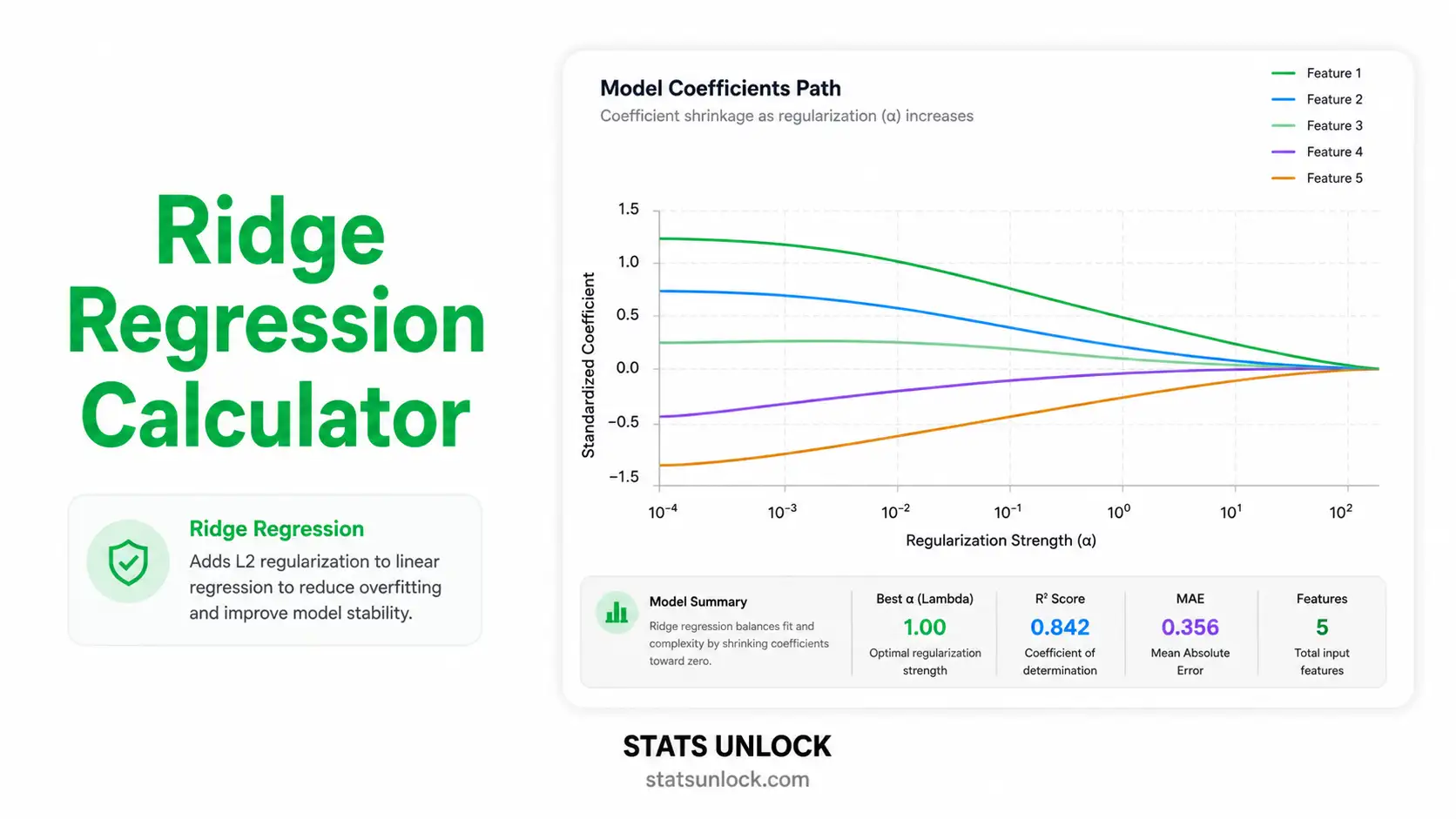
- Examine the Four VisualizationsCoefficient Path: see how each β shrinks as λ grows. CV Error: the U-shape identifies optimal λ. Predicted vs Actual: closeness to the diagonal indicates fit quality. Residuals vs Fitted: should be a random cloud — patterns reveal misspecification.
- Check AssumptionsVIF values in the coefficient table flag multicollinearity. Residual plots reveal heteroscedasticity or nonlinearity. The technical notes section lists every assumption explicitly.
- Read the Detailed InterpretationThe Plain-Language Interpretation Results section gives a multi-paragraph narrative of what the optimal λ means, how each coefficient should be interpreted, what the R² and RMSE imply for prediction, and what the limitations are.
- Export Your ResultsUse Download Doc for a plain-text summary, Download PDF for a print-ready report (browser dialog → Save as PDF), and Copy Summary for a one-paragraph clipboard string ready to paste into a manuscript.
🏁 Conclusion
Ridge regression remains one of the most reliable and widely used methods in the linear modeling toolbox — the bridge between unregularized ordinary least squares and modern machine learning. By adding an L2 penalty to the loss function, ridge stabilizes coefficient estimates whenever predictors are correlated, whenever the number of variables is large relative to the sample size, or whenever out-of-sample prediction matters more than in-sample fit. The result is a model that generalizes better than OLS, retains every predictor in the equation, and produces ranks of variable importance that are reproducible across resamples.
This calculator is built to be a complete teaching and research aid: you can paste raw data, upload a CSV, or enter a manual grid; tune lambda automatically or specify it manually; download polished reports for thesis chapters, peer-reviewed manuscripts, conference posters, and pre-registration documents. Every formula, every assumption, and every interpretation paragraph updates dynamically with your data, so the workflow scales from quick classroom demonstrations to publication-ready analyses.
If your goal is to predict a continuous outcome from many overlapping inputs and you want a model whose coefficients you can defend in a manuscript, ridge regression is almost always a strong default. Combine the diagnostic plots above with the bootstrap standard errors, sanity-check the residuals, and you will have a ridge regression analysis that meets the standards of any peer-reviewed journal — produced in seconds, free, and entirely in your browser.
❓ Frequently Asked Questions
Q1. What is ridge regression and when should I use it?
Ridge regression is a regularized linear regression method that adds an L2 penalty (lambda × sum of squared coefficients) to the ordinary least squares loss function. The penalty shrinks coefficients toward zero, producing a more stable model when predictors are correlated or when the number of predictors is large.
Use it whenever ordinary least squares (OLS) is unstable: high multicollinearity (VIF > 5), too many predictors relative to your sample size, or when out-of-sample prediction matters more than in-sample fit. A common example is house-price prediction from many overlapping property features.
Q2. What is the lambda (λ) parameter in ridge regression?
Lambda is the regularization strength. When λ = 0, ridge regression reduces exactly to OLS. As λ grows, all coefficients shrink toward zero — but ridge (unlike Lasso) almost never sets coefficients to exactly zero.
Larger λ means more shrinkage, lower variance, and slightly higher bias. The optimal λ trades off these two and is found by minimizing cross-validated prediction error. This calculator does that automatically across a 50-point logarithmic grid.
Q3. How does ridge regression handle multicollinearity?
When two or more predictors are highly correlated, the OLS coefficient matrix XᵀX is nearly singular, producing huge, unstable coefficient estimates that flip sign with small changes in the data. Ridge regression adds λI to XᵀX, making it always invertible regardless of correlation structure.
The practical effect: correlated predictors share the explanatory effect more evenly rather than one absorbing all of it and another flipping sign. The result is a model whose coefficients you can actually interpret and whose predictions generalize.
Q4. What is the difference between ridge regression and lasso regression?
Ridge (L2) uses a squared penalty (Σβ²). It shrinks all coefficients smoothly toward zero but rarely makes them exactly zero. Best when you believe most predictors contribute something and you want a stable model.
Lasso (L1) uses an absolute-value penalty (Σ|β|). It can set coefficients to exactly zero, performing automatic feature selection. Best when you suspect only a few predictors truly matter.
If unsure, use Elastic Net, which mixes both penalties.
Q5. Do I need to standardize variables before ridge regression?
Yes. Because the L2 penalty applies equally to all coefficients, predictors must be on the same scale or the penalty will unfairly target variables with larger natural ranges. This calculator standardizes by default (mean 0, SD 1) and converts coefficients back to the original scale for interpretation.
Q6. How do I choose the optimal lambda?
Use k-fold cross-validation. The model is fit on k − 1 folds and evaluated on the held-out fold; the lambda that minimizes the average held-out mean squared error is the optimal one. This calculator runs 10-fold CV across a 50-point log grid spanning 10⁻³ to 10³ by default.
The "1-SE rule" — choosing the largest lambda whose CV error is within one standard error of the minimum — is a common alternative that produces a slightly more parsimonious model.
Q7. What does R-squared mean in ridge regression?
R² is the proportion of variance in the outcome that the model explains. In ridge regression, training R² is computed using shrunken coefficients and is therefore typically slightly lower than OLS R² on the same training data.
The number to trust is the cross-validated R², which estimates how well the model will predict new observations. A ridge model with lower training R² but higher CV R² than OLS is genuinely better.
Q8. Can I get p-values and confidence intervals for ridge coefficients?
Not directly. Ridge produces biased coefficient estimates, so classical OLS p-values and t-tests do not apply. The recommended approach is bootstrap resampling: resample the data 1,000+ times, refit ridge each time, and use the empirical distribution of coefficients to construct confidence intervals.
This calculator reports bootstrap standard errors. Multiply them by 1.96 for an approximate 95% interval.
Q9. Can I use this calculator for my published research or assignment?
Yes — for educational purposes, exploratory analysis, and publication of small studies. For larger studies or clinical/regulatory work, also verify with peer-reviewed software like R's glmnet package or Python's scikit-learn Ridge / RidgeCV.
Cite as: STATS UNLOCK. (2025). Ridge regression calculator. Retrieved from https://statsunlock.com/ridge-regression-calculator
Q10. What if my ridge model has very low R² — is the model wrong?
Not necessarily. Low R² can mean: (a) your predictors genuinely lack information about the outcome, (b) the relationship is nonlinear and ridge cannot capture it, (c) the outcome is intrinsically noisy, or (d) you need additional features.
Diagnose by checking the Residuals vs Fitted plot for nonlinear patterns, comparing ridge to a polynomial or tree-based model, and considering whether you have measured the right predictors. A ridge regression with R² = 0.20 may still be the best linear model possible for the data — and it can still be useful for prediction.
📚 References
📖 References (APA 7th edition)
The following references support the statistical methods used in this ridge regression calculator, covering L2 regularization, cross-validation lambda tuning, and best practices in penalized regression analysis.
- Hoerl, A. E., & Kennard, R. W. (1970). Ridge regression: Biased estimation for nonorthogonal problems. Technometrics, 12(1), 55–67. https://doi.org/10.1080/00401706.1970.10488634
- Hoerl, A. E., & Kennard, R. W. (1970). Ridge regression: Applications to nonorthogonal problems. Technometrics, 12(1), 69–82. https://doi.org/10.1080/00401706.1970.10488635
- Tikhonov, A. N. (1963). Solution of incorrectly formulated problems and the regularization method. Soviet Mathematics Doklady, 4, 1035–1038.
- Hastie, T., Tibshirani, R., & Friedman, J. (2009). The elements of statistical learning: Data mining, inference, and prediction (2nd ed.). Springer. https://doi.org/10.1007/978-0-387-84858-7
- Friedman, J., Hastie, T., & Tibshirani, R. (2010). Regularization paths for generalized linear models via coordinate descent. Journal of Statistical Software, 33(1), 1–22. https://doi.org/10.18637/jss.v033.i01
- James, G., Witten, D., Hastie, T., & Tibshirani, R. (2021). An introduction to statistical learning with applications in R (2nd ed.). Springer. https://doi.org/10.1007/978-1-0716-1418-1
- Tibshirani, R. (1996). Regression shrinkage and selection via the lasso. Journal of the Royal Statistical Society: Series B, 58(1), 267–288. https://doi.org/10.1111/j.2517-6161.1996.tb02080.x
- Zou, H., & Hastie, T. (2005). Regularization and variable selection via the elastic net. Journal of the Royal Statistical Society: Series B, 67(2), 301–320. https://doi.org/10.1111/j.1467-9868.2005.00503.x
- Stone, M. (1974). Cross-validatory choice and assessment of statistical predictions. Journal of the Royal Statistical Society: Series B, 36(2), 111–147. https://doi.org/10.1111/j.2517-6161.1974.tb00994.x
- Efron, B., & Tibshirani, R. J. (1993). An introduction to the bootstrap. Chapman & Hall/CRC. https://doi.org/10.1201/9780429246593
- Cohen, J., Cohen, P., West, S. G., & Aiken, L. S. (2003). Applied multiple regression/correlation analysis for the behavioral sciences (3rd ed.). Lawrence Erlbaum Associates.
- Field, A. (2018). Discovering statistics using IBM SPSS statistics (5th ed.). SAGE Publications.
- American Psychological Association. (2020). Publication manual of the American Psychological Association (7th ed.). APA. https://doi.org/10.1037/0000165-000
- Pedregosa, F., Varoquaux, G., Gramfort, A., et al. (2011). Scikit-learn: Machine learning in Python. Journal of Machine Learning Research, 12, 2825–2830. https://www.jmlr.org/papers/v12/pedregosa11a.html
- R Core Team. (2024). R: A language and environment for statistical computing. R Foundation for Statistical Computing. https://www.R-project.org/


