Weighted Least Squares
(WLS) Calculator
Run weighted least squares regression online. Fix heteroscedasticity, get weighted coefficients, p-values, R², residual diagnostics, and APA-format reporting in seconds.
📊 Step 1 — Enter Your Data
| # | X (Predictor) | Y (Outcome) | Weight (optional) |
|---|
⚙️ Step 2 — Configure Test Settings
🧠 Interpretation Results & How to Write Your Results
📝 How to Write Your Results in Research (5 Examples)
🎯 Conclusion — What Weighted Least Squares Tells You
Weighted Least Squares (WLS) is the most reliable fix for one of the most common problems in linear regression: heteroscedasticity, where the spread of residuals changes systematically with the predictor or fitted value. Ordinary Least Squares (OLS) still produces unbiased coefficients in this situation, but its standard errors, confidence intervals, and p-values become misleading — typically over-stating precision in regions where variance is high. WLS solves this by giving each observation a weight inversely proportional to its variance, so noisy points get less influence and quiet points get more.
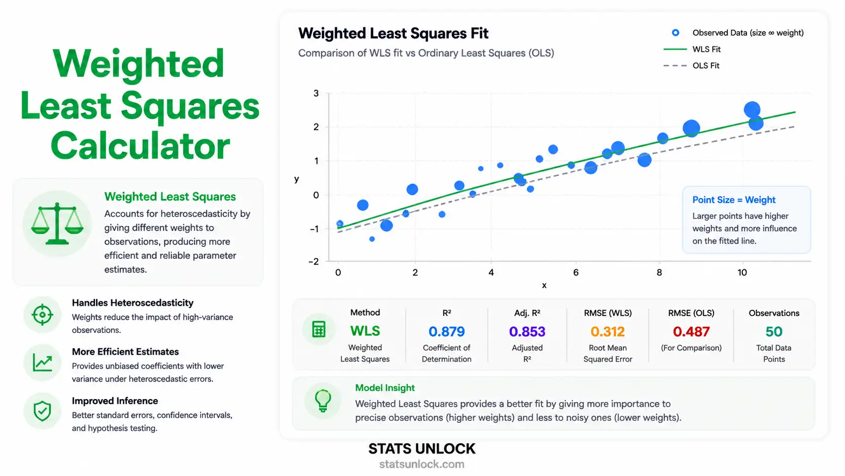
Practical takeaway from this calculator: when you compare a WLS fit to an OLS fit on the same data, three things usually shift in informative ways:
- Coefficients tilt toward the low-variance region. The slope and intercept are pulled by the precise observations and away from the noisy ones.
- Standard errors get more honest. They shrink in regions where data are precise and grow where data are noisy, producing confidence intervals you can actually trust.
- R² drops slightly on the original scale, but the weighted R² (which is what WLS actually optimises) is the correct comparison for a heteroscedastic dataset.
When WLS is the right tool: use it whenever a residuals-vs-fitted plot from an OLS pre-fit fans out, contracts, or shows curved variance bands. It is also the natural choice when observations are aggregated from groups of unequal size (use group n as weight), when each measurement has a known precision (use 1/SE²), or when replicates supply a direct estimate of variance per design point.
When to look further: if errors are not just heteroscedastic but also autocorrelated, you need generalised least squares (GLS). If you suspect non-linearity in addition to heteroscedasticity, transform Y (log, sqrt) or fit a generalised linear model (GLM). If outliers — not variance heterogeneity — are driving the problem, robust regression (M-estimators, Huber, MM) is more appropriate than WLS. WLS is the right tool when the assumption violation is specifically variance heterogeneity, not anything else.
Bottom line: WLS gives you a regression you can defend in peer review when OLS assumptions break in a specific, diagnosable way. Always inspect the residuals from OLS first, choose a weighting scheme that matches the variance pattern you see, and report both the unweighted and weighted statistics so reviewers can verify your decision. This calculator does all of that automatically — including the diagnostic plots, the APA-format reporting strings, and the model-comparison table you need to justify the WLS fit in your paper, thesis, or technical report.
📐 Technical Notes & Formulas Used
Sub-section A — Formulas Used
Sub-section B — Technical Notes
- Linearity: WLS still assumes a linear functional form between X and the conditional mean of Y. WLS only fixes variance, not shape.
- Independence: Errors must be uncorrelated. If autocorrelation is present, use Generalised Least Squares (GLS) instead.
- Heteroscedasticity: WLS targets non-constant variance. Diagnose via residuals-vs-fitted from an OLS pre-fit; choose weights that match the pattern.
- Weight choice matters: the wrong weights can perform worse than OLS. When in doubt, fit OLS, examine residuals, then iterate weights (IRLS).
- No multicollinearity among predictors (only relevant for multiple WLS).
- Sample size: ≥ 20 observations recommended for stable variance estimation; ≥ 50 for inference reliability.
- Robustness: WLS is not robust to outliers — combine with robust regression (M-estimators) if outliers are present alongside heteroscedasticity.
🎯 When to Use Weighted Least Squares
Use WLS when: your residuals from OLS show non-constant variance, when each observation has a known different precision, or when data are aggregated from groups of unequal size and you want to weight by group n.
Decision Checklist
- You have a continuous outcome (Y) and at least one continuous predictor (X)
- Your residuals-vs-fitted plot from OLS shows a fan, funnel, or curved pattern
- You have a defensible weighting scheme (1/x², 1/y², 1/SE², or 1/n)
- Errors are uncorrelated (no autocorrelation)
- The relationship between X and Y is approximately linear
- Do NOT use if errors are autocorrelated → use Generalised Least Squares (GLS)
- Do NOT use if the relationship is non-linear → transform Y or use a GLM
- Do NOT use if the only problem is outliers → use robust regression instead
- Do NOT use without diagnosing variance pattern first → arbitrary weights can hurt
Real-World Examples
1. Economics — Income vs Spending: Spending variance grows with income (richer households have more spending heterogeneity). Use weights = 1/X² to stabilise variance and get reliable elasticity estimates.
2. Pharmacology — Dose-Response Studies: Each dose level is tested with a different number of replicates, and replicate-based variance differs by dose. Use weights = nᵢ / sᵢ² where nᵢ = replicates and sᵢ² = within-dose variance.
3. Agronomy — Fertiliser vs Yield: High-fertiliser plots show greater yield variation due to interactions with soil moisture. Use weights = 1/Ŷ from an OLS pre-fit to down-weight noisy high-fertiliser observations.
4. Ecology — Length-Weight Allometry: Fish weight variance scales with length cubed. Use log-transformed regression with weights = 1/x² in raw scale, or equivalently fit log(weight) ~ log(length) under OLS.
5. Manufacturing — Production Hours vs Output: Quality control measurements have known instrument precision per unit. Use weights = 1/SE² where SE is the reported measurement standard error.
Sample Size Guidance
- n ≥ 20: Minimum for stable WLS coefficient estimates
- n ≥ 50: Recommended for reliable standard errors and p-values
- n ≥ 100: Required for variance-pattern diagnostics (OLS residual smoothing)
Decision Tree — WLS vs Alternatives
📖 How to Use This Weighted Least Squares Calculator
- Step 1 — Enter Your Data
Three options: type/paste comma-separated X and Y values, upload a CSV/Excel file (with column picker), or use the manual table. The calculator pre-loads the "Income vs Spending" sample (n = 15) so you can see results instantly. Example: X = "25, 32, 41, …", Y = "22, 27, 35, …"
- Step 2 — Choose a Sample Dataset (optional)
Five built-in datasets are provided: Income vs Spending (variance grows with X), Drug Dose vs Response, Fertiliser vs Yield, Fish Length vs Weight (allometric), and Production Hours vs Output. Each is pre-configured with realistic heteroscedasticity so you can compare WLS to OLS on the same data.
- Step 3 — Configure the Weighting Scheme
Pick a weighting scheme from the dropdown: 1/X (variance ∝ X), 1/X² (variance ∝ X²), 1/Ŷ, 1/Ŷ², 1/residual² (from an OLS pre-fit — fully automatic), Equal weights (reproduces OLS), or Custom (you supply weights). The 1/residual² option is the most flexible — it does not require you to guess the variance pattern.
- Step 4 — Set Test Settings
Choose α (0.01, 0.05, or 0.10), include or exclude the intercept, and pick decimal precision (2–5 places). 95% confidence is the default and matches APA reporting conventions.
- Step 5 — Click "Run WLS Analysis"
The calculator computes WLS coefficients, weighted R², F-statistic, t-statistics, p-values, and confidence intervals — and also runs an OLS comparison automatically.
- Step 6 — Read the Summary Cards
The four cards at the top show: Slope (β₁), Intercept (β₀), Weighted R², and p-value of the slope. Green = significant, amber = borderline, red = non-significant.
- Step 7 — Read the Full Results Table
The detailed table shows every coefficient with its SE, t-statistic, p-value, 95% CI, and a description. The model fit row shows F, df, R²_w, and the residual standard error.
- Step 8 — Examine Both Visualisations
The first plot is a scatter with WLS and OLS lines overlaid, with point sizes proportional to weights — so you can see which observations dominate the fit. The second plot is the residuals-vs-fitted diagnostic — flat band = WLS worked, fan = try a different weighting scheme.
- Step 9 — Read the Interpretation
The plain-language interpretation block translates the numbers into sentences you can paste into a Methods or Results section. The five reporting examples (APA, Thesis, Plain-Language, Conference Abstract, Pre-Registration) auto-fill with your statistics.
- Step 10 — Export Your Results
Click Download Doc for a plain-text .txt report (paste into Word/Google Docs), or Download PDF for a print-ready PDF with all 8 sections and the StatsUnlock branded footer.
❓ Frequently Asked Questions
Q1. What is weighted least squares (WLS) and when should I use it?
WLS is a regression method that assigns different weights to observations to correct for heteroscedasticity (non-constant error variance). Use it when residuals from an OLS fit show a fan, funnel, or curved pattern, when each observation has a known different precision, or when data are aggregated from groups of unequal size.
Q2. How is WLS different from OLS?
OLS minimises Σ(yᵢ − ŷᵢ)² — every residual counts equally. WLS minimises Σ wᵢ(yᵢ − ŷᵢ)² — observations with higher weight (lower variance) count more. When all weights are equal, WLS reduces exactly to OLS.
Q3. How do I choose the right weights?
The optimal weight is wᵢ = 1/σᵢ² where σᵢ² is the variance of the error at observation i. In practice you estimate the variance pattern from an OLS pre-fit: if residuals fan out with X, use 1/X or 1/X²; if they fan out with Ŷ, use 1/Ŷ or 1/Ŷ²; if you have replicates, use replicate-based variance. The "1/residual²" option in this calculator does this automatically.
Q4. Will WLS give different coefficients than OLS?
Yes — when weights are non-uniform. WLS coefficients are pulled toward the low-variance (high-weight) observations and away from the high-variance (low-weight) ones. The bigger the variance heterogeneity, the bigger the difference between WLS and OLS estimates.
Q5. What is weighted R² and how do I interpret it?
Weighted R² = 1 − Σ wᵢ(yᵢ − ŷᵢ)² / Σ wᵢ(yᵢ − ȳ_w)². It is the proportion of weighted variance in Y explained by the model. It is the correct R² to report for WLS — not the unweighted R² calculated on the original scale.
Q6. How do I report WLS results in APA format?
Report the weighting scheme, the F-statistic with df, the weighted R², and the slope's β, SE, t, and p. Example: "A weighted least squares regression with weights = 1/X was conducted; the model was significant, F(1, 13) = 142.6, p < .001, R²_w = .916, β = 1.03, SE = 0.09, t = 11.94, p < .001."
Q7. Can WLS handle multiple predictors (multiple WLS)?
Yes — WLS extends naturally with X as an n×p design matrix and W as an n×n diagonal weight matrix. The matrix formula β̂ = (XᵀWX)⁻¹XᵀWy works identically. This calculator focuses on simple WLS (one predictor) for clarity and visualisation, but the math is the same.
Q8. What if I do not know the variance pattern?
Run OLS first, plot residuals vs fitted values, and identify the variance pattern visually (fan, funnel, megaphone). If the pattern is unclear, use the "1/residual²" option in this calculator — it automates iterative reweighted least squares (IRLS) by using OLS residuals to estimate variance.
Q9. Is WLS the same as generalised least squares (GLS)?
WLS is a special case of GLS where the error covariance matrix Σ is diagonal (uncorrelated errors with different variances). GLS allows full covariance matrices for autocorrelated errors. If your errors are correlated (e.g., time-series, clustered data), use GLS or mixed models, not WLS.
Q10. Can WLS handle outliers?
Not directly. WLS is designed for heteroscedasticity, not outliers. If outliers are the issue, use robust regression (M-estimators, Huber, MM). If you have both heteroscedasticity AND outliers, combine the two: weighted M-estimation, or transform the outcome first (log, Box-Cox) and then run OLS.
📚 References
The following references support the statistical methods used in this weighted least squares calculator, covering heteroscedasticity correction, weighted regression analysis, and best practices in p-value interpretation and effect size reporting for WLS regression.
- Aitken, A. C. (1936). On least squares and linear combinations of observations. Proceedings of the Royal Society of Edinburgh, 55, 42–48. https://doi.org/10.1017/S0370164600014346
- Carroll, R. J., & Ruppert, D. (1988). Transformation and weighting in regression. Chapman and Hall. https://doi.org/10.1201/9780203735268
- White, H. (1980). A heteroskedasticity-consistent covariance matrix estimator and a direct test for heteroskedasticity. Econometrica, 48(4), 817–838. https://doi.org/10.2307/1912934
- Breusch, T. S., & Pagan, A. R. (1979). A simple test for heteroscedasticity and random coefficient variation. Econometrica, 47(5), 1287–1294. https://doi.org/10.2307/1911963
- Greene, W. H. (2018). Econometric analysis (8th ed.). Pearson.
- Weisberg, S. (2014). Applied linear regression (4th ed.). John Wiley & Sons. https://doi.org/10.1002/9781118625590
- Fox, J. (2016). Applied regression analysis and generalized linear models (3rd ed.). SAGE Publications.
- Long, J. S., & Ervin, L. H. (2000). Using heteroscedasticity consistent standard errors in the linear regression model. The American Statistician, 54(3), 217–224. https://doi.org/10.1080/00031305.2000.10474549
- Cribari-Neto, F., & Zarkos, S. G. (1999). Bootstrap methods for heteroskedastic regression models: Evidence on estimation and testing. Econometric Reviews, 18(2), 211–228. https://doi.org/10.1080/07474939908800440
- Cohen, J. (1988). Statistical power analysis for the behavioral sciences (2nd ed.). Lawrence Erlbaum Associates.
- American Psychological Association. (2020). Publication manual of the American Psychological Association (7th ed.). APA. https://doi.org/10.1037/0000165-000
- R Core Team. (2024). R: A language and environment for statistical computing. R Foundation for Statistical Computing. https://www.R-project.org/
- NIST/SEMATECH. (2013). e-Handbook of statistical methods. National Institute of Standards and Technology. https://www.itl.nist.gov/div898/handbook/
- Seabold, S., & Perktold, J. (2010). statsmodels: Econometric and statistical modeling with Python. Proceedings of the 9th Python in Science Conference, 92–96. https://doi.org/10.25080/Majora-92bf1922-011
- Faraway, J. J. (2014). Linear models with R (2nd ed.). Chapman and Hall/CRC. https://doi.org/10.1201/b17144


