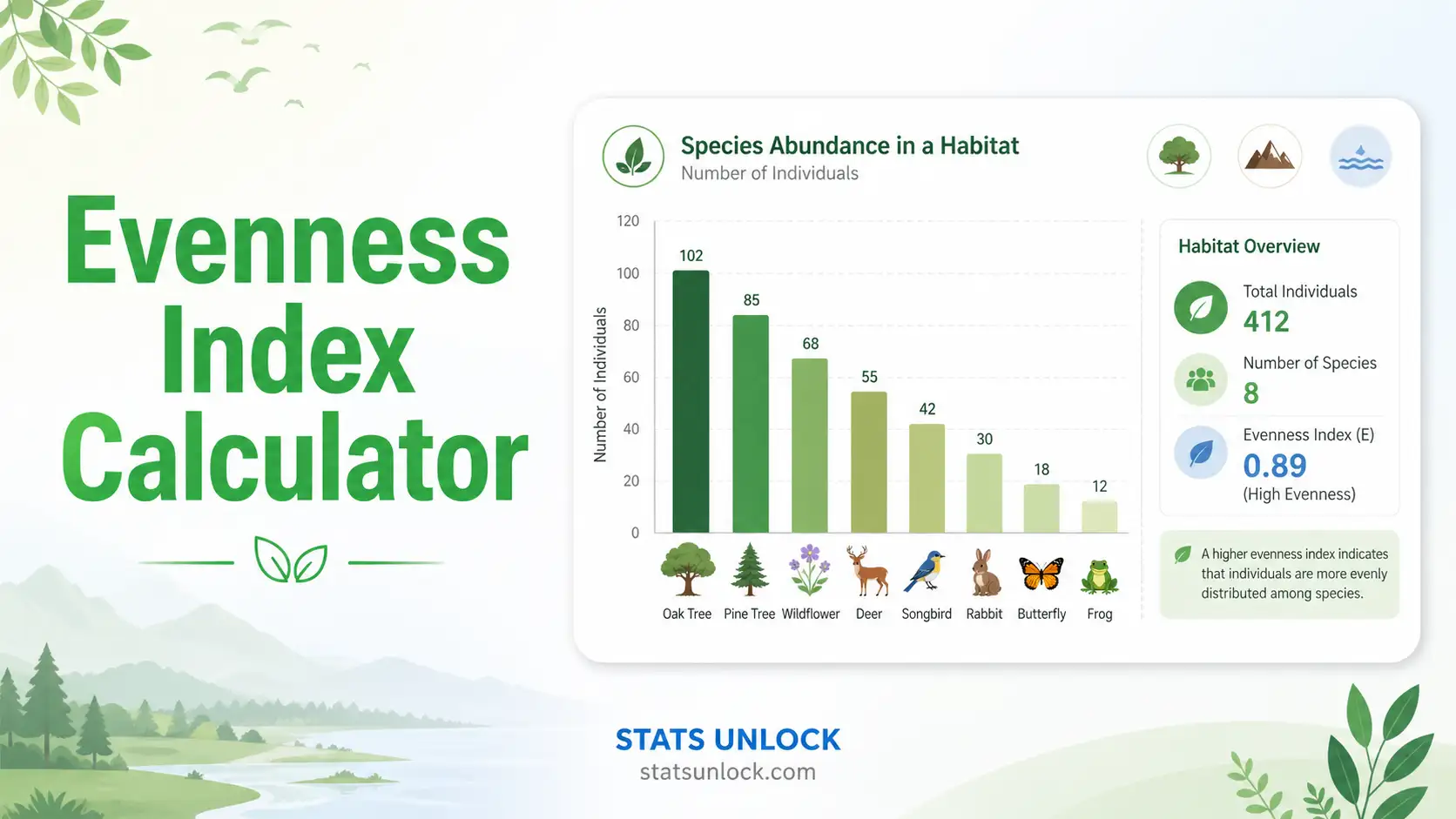
Evenness Index Calculator
A free online tool to measure species evenness with Pielou's J', Simpson's evenness, Heip's index, and Evar from your survey counts, with instant charts and report-ready results.
⚡ 0. Quick Answer
The evenness index calculator shows how equally individuals are shared among species, on a scale of 0 to 1. Enter counts such as 45, 30, 15, 7, 3 and the tool returns Pielou's J' = 0.806 from J' = H' / ln S, plus Simpson's evenness 0.623, Heip's 0.664 and Smith and Wilson's Evar 0.514.
🌿 Key Takeaways
- The evenness index calculator shows how equally individuals are spread across species, from balanced to strongly dominated.
- You only need the count of individuals per species. Paste them comma separated, upload a CSV file, or type them in.
- It returns Pielou's evenness (J'), Simpson's evenness, Heip's evenness, and the Evar index, all on a 0 to 1 scale.
- A value near 1 means all species are similarly common; a value near 0 means one or a few species dominate.
- Typical field uses: camera trapping, point counts, vegetation plots, transects, and reef fish surveys.
🌱 1. What Is Species Evenness?
Species evenness describes how equally individuals are shared among the species present. It is the half of biodiversity that a species list cannot show you. Richness asks how many species there are. Evenness asks whether they are balanced or whether one species holds nearly everything.
Every evenness index works the same way underneath: it compares the diversity you actually measured against the diversity you would have seen if every species were equally common. Pielou's J', the standard, divides the Shannon index by its maximum possible value, ln S. The answer runs from 0 to 1, where 1 means perfectly even.
This matters because evenness usually changes before richness does. When a habitat starts to degrade, or an invasive species arrives, the species list often stays the same for years while the balance between species shifts underneath it. Evenness picks that up first, which makes it one of the earliest warning signals in monitoring work.
1.1 The four evenness indices this tool reports
| Index | Formula | Built on | Use it when |
|---|---|---|---|
| Pielou's evenness (J') | H' / ln S | Shannon index | The default. Report this unless you have a reason not to. |
| Simpson's evenness (E1/D) | (1/D) / S | Simpson's index | Dominance is your question; it leans on common species. |
| Heip's evenness | (eH' - 1) / (S - 1) | Shannon index | You are comparing sites with different richness. |
| Smith and Wilson Evar | 1 - (2/π) arctan(variance of ln n) | Raw counts | You want an index genuinely independent of richness. |
What to conclude: the four indices will not agree, and they are not meant to. On this page's worked example they range from 0.514 to 0.806 for the same data. Pick one, name it, and use it consistently across every site in your study.
1.2 What the value means
| Pielou's J' | Reading | Typical setting |
|---|---|---|
| 0.90 to 1.00 | Very even Healthy | Stable, undisturbed communities; well-sampled insect traps |
| 0.75 to 0.90 | Even Healthy | Mature forest, healthy reef, good grassland |
| 0.60 to 0.75 | Moderate Watch | Secondary forest, managed land, seasonal aggregations |
| 0.40 to 0.60 | Uneven Watch | Disturbed sites, early succession, feeding congregations |
| Below 0.40 | Very uneven Concern | Invasion, pollution, monoculture, heavy management |
What to conclude: a low evenness value is not automatically bad. Some natural systems, such as reed beds, salt marshes and breeding colonies, are genuinely dominated by one species. Compare against a reference site before calling it degradation.
📥 2. Set Up Your Data
0 values entered
🔎 4. Interpretation of Results, In Detail
▶ Run the analysis above to generate a detailed, plain-English interpretation of your evenness result.
✍️ 5. How to Write Your Results in Research
▶ Run the analysis above to auto-fill all six examples with your results.
🪧 5.1 Research Poster Panel
A print-ready poster layout that updates with your result. Copy the text or use the visual scaffold for A0 / A1 conference posters.
▶ Run the analysis above to build your poster panel.
🧮 6. Formulas Used
Every number this evenness index calculator reports comes from one of the seven formulas below. Cards 1 and 2 build the inputs, cards 3 to 6 are the four evenness indices, and card 7 is the quick dominance check.
Shannon index, the input to most evenness measures
- H' Shannon Wiener index, unitless
- pi proportion of individuals in species i, ni divided by N
- Example: counts 45, 30, 15, 7, 3 give H' = 1.296.
- Requires: raw counts, not percentages.
Maximum possible diversity
- S species richness, a count
- Meaning: the value H' would take if every species were equally common.
- Example: ln 5 = 1.609.
- Note: this is the denominator that turns diversity into evenness.
Pielou's evenness, the standard
- J' evenness, unitless, 0 to 1
- Range: 1.0 is perfectly even, values under 0.5 mean strong dominance.
- Example: 1.296 / 1.609 = 0.806.
- Note: undefined when S = 1, because ln 1 = 0. A single species has no evenness.
Simpson's evenness
- 1/D Simpson's reciprocal index, the effective number of common species
- Range: 0 to 1.
- Example: 3.117 / 5 = 0.623.
- Use for: when dominance by common species is the question. It ignores rare species almost entirely.
Heip's evenness
- Range: 0 to 1.
- Example: (3.656 - 1) / 4 = 0.664.
- Use for: comparing sites whose species richness differs, because it is less pulled by S than J' is.
- Note: undefined when S = 1.
Smith and Wilson's Evar
- ni the raw count of species i, not its proportion
- Range: 0 to 1.
- Example: variance of the logged counts is 0.958, so Evar = 0.514.
- Use for: the one index genuinely independent of richness. It is the purest evenness measure here.
Berger-Parker dominance, the quick check
- nmax count of the single commonest species
- Example: 45 / 100 = 0.45, so the top species holds 45 percent of individuals.
- Use for: a one-second sanity check. High d always means low evenness.
🧭 7. How to Use This Calculator
Ten steps from a field sheet to a publication-ready evenness result.
- Collect standardised counts. Record the number of individuals for each species using the same effort at every site.
- Count individuals, not just species. Evenness is impossible from a presence-only species list.
- Pick an input tab. Use Paste or Type for a quick run, Upload CSV for a spreadsheet, or Manual Table to key in rows.
- Enter species names and counts. In Column Entry mode, put the species name on the left and the count on the right.
- Or load a sample dataset. Choose one of the built-in field datasets to see how the tool behaves before you use your own data.
- Name your study area. Type the site name into the Study Area box so it appears in every report template and in the poster panel.
- Choose which index to highlight. Pielou's J' is the default and the one most journals expect.
- Click Run Analysis. The tool returns all four evenness indices, richness, the Shannon index, charts and a results table.
- Read across the four indices. If they disagree sharply, your community has an unusual abundance shape, which is worth a sentence in your results.
- Copy or download your result. Use the report templates, the poster panel, Download Doc or Download PDF for your thesis or paper.
📗 8. How to Calculate Species Evenness in Excel
Excel, step by step, with the same worked example used everywhere on this page
The worked example below uses five species with counts 45, 30, 15, 7, 3 (N = 100). Excel, R, Python and this calculator all return Pielou's J' = 0.806, Simpson's evenness 0.623, Heip's 0.664 and Evar 0.514 for it.
8.1 The Excel functions you need
| Function | What it does | Example |
|---|---|---|
| SUMPRODUCT | Builds the Shannon index in one cell | =-SUMPRODUCT(C2:C6,LN(C2:C6)) |
| LN | Natural logarithm, used for H', ln S and Evar | =LN(COUNTIF(B2:B6,">0")) |
| COUNTIF | Counts species present, giving S | =COUNTIF(B2:B6,">0") |
| SUMSQ | Sum of squared proportions, the input to Simpson's evenness | =SUMSQ(C2:C6) |
| VAR.P | Population variance of the logged counts, for Evar | =VAR.P(E2:E6) |
| ATAN and PI | The arctangent step in Smith and Wilson's Evar | =1-(2/PI())*ATAN(VAR.P(E2:E6)) |
What to conclude: the only unusual function here is VAR.P. Use the population form, not VAR.S, or your Evar will be slightly too low.
8.2 Step by step in the sheet
Step 1. Turn counts into proportions
Species names in column A, counts in column B, and C2 holds =B2/$B$7, returning 0.45. The dollar signs lock the total so the formula fills down to C6. Column C now adds to 1.00.
Step 2. Build the Shannon index
Column D holds =C2*LN(C2) for each row, and D7 totals them with the sign flipped: =-SUMPRODUCT(C2:C6,LN(C2:C6)) returns H' = 1.2964. Evenness needs this number first.
Step 3. Divide by ln S to get Pielou's evenness
D8 holds =D7/LN(COUNTIF(B2:B6,">0")) and returns J' = 0.8055. Using COUNTIF inside the formula means the sheet still works when you add or remove species rows.
Step 4. Add Evar, the richness-independent index
Column E holds =LN(B2), the natural log of the raw count rather than the proportion. E7 returns Evar = 0.5136. Note the input is the count, not the proportion: this is the mistake that breaks Evar most often.
8.3 The awkward cases
| Case | What breaks | Fix |
|---|---|---|
| Only one species (S = 1) | ln 1 = 0, so J' divides by zero | Evenness is undefined for one species. Report richness instead. |
| A species with a count of 0 | LN(0) returns #NUM! and inflates S | Delete the row before calculating |
| Evar fed with proportions | Returns a wrong value silently, with no error | Evar takes raw counts. Point column E at column B, not column C. |
| VAR.S used instead of VAR.P | Evar comes out slightly too low | Use VAR.P, the population form, as the published definition specifies |
| Counts entered as percentages | J' still works, Evar does not | Go back to raw counts if you need Evar |
What to conclude: J' tolerates proportions, Evar does not. That single difference causes most of the mismatched evenness values people report.
8.4 Why answers differ between Excel, R and Python
Nearly always because a different evenness index was used. R's vegan has no single "evenness" function: J' is written by hand as diversity(x)/log(specnumber(x)), while Evar comes from a separate helper. If someone quotes 0.623 and you have 0.806, you are almost certainly comparing Simpson's evenness against Pielou's on the same data. The second cause is the log base: J' is a ratio, so it is unaffected by whether you use ln or log2 as long as you use the same base top and bottom, but mixing bases within the fraction produces nonsense. Rounding proportions before summing is the third and smallest cause.
8.5 Charting the result in Excel
- Rank abundance curve. Sort counts largest to smallest and Insert a Line chart. The steepness of the line is evenness, made visible.
- Four-index comparison bars. Chart J', Simpson's E, Heip's and Evar side by side. Where they diverge tells you about the shape of your community.
- Evenness across sites. One J' value per site in a clustered bar chart, with the axis fixed 0 to 1 so differences are not exaggerated.
- Label the axis with the index name. Write "Pielou's J'" rather than "evenness", because four different numbers answer to that word.
8.6 Excel error messages and what they mean
| Message | Cause | Fix |
|---|---|---|
| #DIV/0! | S = 1, so ln S is zero | Evenness needs at least two species |
| #NUM! | LN of zero or a negative number | Remove zero counts before calculating |
| #VALUE! | Text inside a numeric range | Clear notes such as "none seen" from the count column |
| Result above 1 | The wrong denominator, usually S instead of ln S | Evenness cannot exceed 1. Check the ln. |
| Result is exactly 1 | Every species has an identical count | Correct. That is perfect evenness. |
| Evar is negative | ATAN applied to something other than a variance | Check that VAR.P points at the logged counts |
What to conclude: any evenness value outside 0 to 1 is an arithmetic error, not a finding.
📘 9. How to Calculate Species Evenness in R
R, one complete script you can run top to bottom
9.1 The complete script
Copy this into RStudio and press Run. It needs no packages. Change only the counts line. It prints all four evenness indices and saves one 300 dpi figure.
# ------------------------------------------------------------------
# Species Evenness Indices in R
# StatsUnlock.com - free ecology and wildlife analysis tools
# ------------------------------------------------------------------
set.seed(42)

# 1. YOUR DATA -- change only this line
counts <- c(45, 30, 15, 7, 3)
species <- c("Bulbul", "Babbler", "Sunbird", "Barbet", "Drongo")

# Reading from a file instead? Uncomment the two lines below.
# dat <- read.csv("my_survey.csv")          # columns: species, count
# counts <- dat$count; species <- dat$species

# 2. CLEAN THE DATA
counts[is.na(counts)] <- 0        # missing values become zero
keep <- counts > 0                # drop zero counts, ln(0) is undefined
counts <- counts[keep]
species <- species[keep]

# 3. CALCULATE
N <- sum(counts)                          # total individuals
S <- length(counts)                       # species richness
p <- counts / N                           # proportions
H <- -sum(p * log(p))                     # Shannon index
Hmax <- log(S)                            # maximum possible diversity

pielou <- H / Hmax                        # Pielou's J', the standard
invD <- 1 / sum(p^2)                      # Simpson's reciprocal index
simpsonE <- invD / S                      # Simpson's evenness
heip <- (exp(H) - 1) / (S - 1)            # Heip's evenness
lnc <- log(counts)                        # Evar uses RAW counts, not proportions
varln <- sum((lnc - mean(lnc))^2) / S     # population variance
evar <- 1 - (2 / pi) * atan(varln)        # Smith and Wilson's Evar
berger <- max(counts) / N                 # Berger-Parker dominance

# The vegan package has no single evenness function. Build J' like this:
# install.packages("vegan")
# library(vegan)
# pielou <- vegan::diversity(counts) / log(vegan::specnumber(counts))

# 4. PRINT A PLAIN-ENGLISH VERDICT
verdict <- if (pielou >= 0.80) "high evenness" else
           if (pielou >= 0.50) "moderate evenness" else "low evenness, dominance present"
cat("Species richness S      :", S, "\n")
cat("Total individuals N     :", N, "\n")
cat("Shannon H'              :", round(H, 3), "\n")
cat("Pielou's evenness J'    :", round(pielou, 3), "\n")
cat("Simpson's evenness      :", round(simpsonE, 3), "\n")
cat("Heip's evenness         :", round(heip, 3), "\n")
cat("Smith & Wilson Evar     :", round(evar, 3), "\n")
cat("Berger-Parker dominance :", round(berger, 3), "\n")
cat("Verdict                 :", verdict, "\n")

# 5. SAVE ONE 300 dpi FIGURE
png("evenness_indices.png", width = 1800, height = 1200, res = 300)
vals <- c(pielou, simpsonE, heip, evar)
bp <- barplot(vals,
              names.arg = c("Pielou J'", "Simpson E", "Heip", "Evar"),
              col = c("#27a558", "#2b7fd4", "#8b5cf6", "#d97706"),
              border = NA, ylim = c(0, 1),
              ylab = "Evenness (0 to 1)",
              main = paste0("Evenness indices, J' = ", round(pielou, 3)))
text(bp, vals, labels = round(vals, 3), pos = 3, cex = 0.9)
dev.off()
cat("Figure saved as evenness_indices.png\n")
9.2 What each line does
| Line | What it does |
|---|---|
| counts <- c(45, 30, ...) | Your species counts. This is the only line most users change. |
| keep <- counts > 0 | Drops zero counts. They break the log and inflate S. |
| H <- -sum(p * log(p)) | The Shannon index, which three of the four evenness indices need. |
| Hmax <- log(S) | Maximum possible diversity, the denominator of Pielou's J'. |
| pielou <- H / Hmax | Pielou's evenness, the index most journals expect. |
| simpsonE <- invD / S | Simpson's evenness, weighted toward common species. |
| heip <- (exp(H) - 1) / (S - 1) | Heip's evenness, less influenced by richness than J'. |
| lnc <- log(counts) | Evar runs on raw counts, not proportions. This line is where people go wrong. |
| varln <- sum(...) / S | Population variance. Note the divisor is S, not S - 1, so do not use var(). |
| evar <- 1 - (2/pi) * atan(varln) | Smith and Wilson's Evar, the richness-independent index. |
| diversity(x) / log(specnumber(x)) | How to build J' with vegan. There is no single evenness function in the package. |
9.3 What the figure shows
The script saves all four evenness indices as labelled bars on a fixed 0 to 1 axis. That fixed axis matters: evenness values are bounded, so a free axis exaggerates small differences and misleads readers. When the four bars sit close together your community has an ordinary abundance shape. When Evar sits far below J', as it does here at 0.514 against 0.806, a few species are much commoner than the rest.
9.4 Problems and fixes
| Problem | Cause | Fix |
|---|---|---|
| Error: could not find function "evenness" | vegan has no evenness function | Build it: diversity(x) / log(specnumber(x)) |
| J' returns NaN | S = 1, so log(S) is zero | Evenness is undefined for a single species |
| Evar does not match this page | var() was used, which divides by S - 1 | Use the population variance, dividing by S, as in the script |
| Evar looks wrong but throws no error | Proportions were passed instead of raw counts | Evar takes counts. Check the log() input. |
| Two indices disagree sharply | Expected behaviour, not a bug | They weight common and rare species differently. Report which one you used. |
| Empty PNG file | dev.off() was never called | Run dev.off() once, then re-run the plotting block |
9.5 One-liners worth keeping
| Code | Returns |
|---|---|
| vegan::diversity(x) / log(vegan::specnumber(x)) | Pielou's J' from a vector or a site-by-species matrix |
| vegan::diversity(x, "invsimpson") / vegan::specnumber(x) | Simpson's evenness |
| (exp(vegan::diversity(x)) - 1) / (vegan::specnumber(x) - 1) | Heip's evenness |
| max(x) / sum(x) | Berger-Parker dominance |
| vegan::rankabundance(x) | The rank abundance table behind the evenness picture |
| vegan::radfit(x) | Fits abundance models to describe the community shape |
🐍 10. How to Calculate Species Evenness in Python
Python, one complete script you can run top to bottom
10.1 The complete script
Save this as evenness.py and run it. Change only the counts line. It prints all four evenness indices and saves one 300 dpi figure.
# ------------------------------------------------------------------
# Species Evenness Indices in Python
# StatsUnlock.com - free ecology and wildlife analysis tools
# ------------------------------------------------------------------
import numpy as np
import matplotlib
matplotlib.use("Agg")
import matplotlib.pyplot as plt

np.random.seed(42)

# 1. YOUR DATA -- change only this line
counts = np.array([45, 30, 15, 7, 3], dtype=float)
species = ["Bulbul", "Babbler", "Sunbird", "Barbet", "Drongo"]

# Reading from a file instead? Uncomment the three lines below.
# import pandas as pd
# dat = pd.read_csv("my_survey.csv")          # columns: species, count
# counts, species = dat["count"].to_numpy(float), dat["species"].tolist()

# 2. CLEAN THE DATA
counts = np.nan_to_num(counts, nan=0.0)       # missing values become zero
keep = counts > 0                             # drop zero counts, log(0) undefined
species = [s for s, k in zip(species, keep) if k]
counts = counts[keep]

# 3. CALCULATE
N = counts.sum()                              # total individuals
S = counts.size                               # species richness
p = counts / N                                # proportions
H = float(-np.sum(p * np.log(p)))             # Shannon index
Hmax = np.log(S)                              # maximum possible diversity

pielou = H / Hmax                             # Pielou's J', the standard
invD = 1 / np.sum(p ** 2)                     # Simpson's reciprocal index
simpson_e = invD / S                          # Simpson's evenness
heip = (np.exp(H) - 1) / (S - 1)              # Heip's evenness
lnc = np.log(counts)                          # Evar uses RAW counts, not proportions
varln = np.sum((lnc - lnc.mean()) ** 2) / S   # population variance
evar = 1 - (2 / np.pi) * np.arctan(varln)     # Smith and Wilson's Evar
berger = counts.max() / N                     # Berger-Parker dominance

# SciPy shortcut for the Shannon step:
# from scipy.stats import entropy
# H = entropy(counts)          # natural log by default

# 4. PRINT A PLAIN-ENGLISH VERDICT
if pielou >= 0.80:
    verdict = "high evenness"
elif pielou >= 0.50:
    verdict = "moderate evenness"
else:
    verdict = "low evenness, dominance present"
print(f"Species richness S      : {S}")
print(f"Total individuals N     : {N:.0f}")
print(f"Shannon H'              : {H:.3f}")
print(f"Pielou's evenness J'    : {pielou:.3f}")
print(f"Simpson's evenness      : {simpson_e:.3f}")
print(f"Heip's evenness         : {heip:.3f}")
print(f"Smith & Wilson Evar     : {evar:.3f}")
print(f"Berger-Parker dominance : {berger:.3f}")
print(f"Verdict                 : {verdict}")

# 5. SAVE ONE 300 dpi FIGURE
labels = ["Pielou J'", "Simpson E", "Heip", "Evar"]
vals = [pielou, simpson_e, heip, evar]
fig, ax = plt.subplots(figsize=(6, 4))
bars = ax.bar(labels, vals, color=["#27a558", "#2b7fd4", "#8b5cf6", "#d97706"])
ax.bar_label(bars, fmt="%.3f", padding=3)
ax.set_ylim(0, 1)
ax.set_ylabel("Evenness (0 to 1)")
ax.set_title(f"Evenness indices, J' = {pielou:.3f}")
plt.tight_layout()
plt.savefig("evenness_indices.png", dpi=300)
print("Figure saved as evenness_indices.png")
10.2 What each line does
| Line | What it does |
|---|---|
| matplotlib.use("Agg") | Draws without a screen, so the script runs on a server or in a notebook. |
| counts = np.array([...]) | Your species counts. The only line most users change. |
| keep = counts > 0 | Drops zero counts, which would send np.log to negative infinity. |
| H = -np.sum(p * np.log(p)) | The Shannon index, needed by three of the four evenness measures. |
| Hmax = np.log(S) | Maximum possible diversity, the denominator of Pielou's J'. |
| pielou = H / Hmax | Pielou's evenness, the standard index. |
| simpson_e = invD / S | Simpson's evenness, weighted toward common species. |
| heip = (np.exp(H) - 1) / (S - 1) | Heip's evenness, less pulled by species richness. |
| lnc = np.log(counts) | Evar takes raw counts, not proportions. The commonest mistake in this script. |
| varln = np.sum(...) / S | Population variance. NumPy's var() already divides by S, unlike R's var(). |
| ax.set_ylim(0, 1) | Fixes the axis, because evenness is bounded and a free axis misleads. |
10.3 What the figure shows
The saved PNG shows the four indices as labelled bars on a fixed 0 to 1 axis, identical in meaning to the R figure. For the rank abundance picture instead, sort the counts descending and plot them on a log y axis: the slope of that line is what every evenness index is summarising into one number.
10.4 Problems and fixes
| Problem | Cause | Fix |
|---|---|---|
| skbio pielou_e differs slightly | scikit-bio uses base 2 in some versions | J' is a ratio, so the base cancels only if used top and bottom. Check the docstring. |
| RuntimeWarning: divide by zero | A zero count reached np.log | Keep the counts > 0 filter |
| J' returns nan | S = 1, so np.log(S) is zero | Evenness is undefined for a single species |
| Evar disagrees with R | R's var() divides by S - 1, NumPy's var() divides by S | Use the population form in both. The script does this explicitly. |
| Evar looks wrong with no error | Proportions passed instead of raw counts | Evar takes counts. Check the np.log input. |
| Figure window never opens | The Agg backend has no screen output | That is expected. Open the saved PNG file. |
10.5 One-liners worth keeping
| Code | Returns |
|---|---|
| skbio.diversity.alpha.pielou_e(c) | Pielou's evenness from integer counts |
| entropy(c) / np.log((c > 0).sum()) | Pielou's J' using SciPy for the Shannon step |
| (1/np.sum((c/c.sum())**2)) / (c > 0).sum() | Simpson's evenness |
| (np.exp(entropy(c)) - 1) / ((c > 0).sum() - 1) | Heip's evenness |
| 1 - (2/np.pi)*np.arctan(np.log(c).var()) | Smith and Wilson's Evar, since NumPy var() is already the population form |
| c.max() / c.sum() | Berger-Parker dominance |
📋 11. Reference Tables
Six lookup tables for reading, comparing and sanity-checking a species evenness result.
Table 11.1 Published Pielou's J' values by habitat type
| Habitat | Taxon | Typical J' | Typical S |
|---|---|---|---|
| Lowland tropical rainforest | Birds | 0.80 to 0.92 | 40 to 120 |
| Dry deciduous forest | Birds | 0.75 to 0.88 | 25 to 50 |
| Temperate woodland | Birds | 0.72 to 0.86 | 15 to 35 |
| Grassland, managed | Plants | 0.60 to 0.82 | 10 to 30 |
| Wetland, freshwater | Waterbirds | 0.65 to 0.85 | 12 to 40 |
| Coral reef transect | Fish | 0.75 to 0.90 | 30 to 80 |
| Camera trap grid | Large mammals | 0.60 to 0.85 | 6 to 20 |
| Urban park | Birds | 0.55 to 0.80 | 8 to 20 |
| Intensive cropland | Arthropods | 0.45 to 0.72 | 5 to 20 |
| Reed bed or breeding colony | Birds | 0.20 to 0.50 | 3 to 15 |
What to conclude: note the last row. A breeding colony is naturally dominated by one species and scores very low, yet it may be the most valuable site in the region. Low evenness is not the same as poor habitat.
Table 11.2 The four indices on the same five datasets
| Counts | Pielou J' | Simpson E | Heip | Evar |
|---|---|---|---|---|
| 20, 20, 20, 20, 20 | 1.000 | 1.000 | 1.000 | 1.000 |
| 45, 30, 15, 7, 3 | 0.806 | 0.623 | 0.664 | 0.514 |
| 40, 30, 20, 8, 2 | 0.826 | 0.674 | 0.695 | 0.448 |
| 80, 5, 5, 5, 5 | 0.483 | 0.308 | 0.294 | 0.435 |
| 96, 1, 1, 1, 1 | 0.139 | 0.217 | 0.063 | 0.186 |
What to conclude: all four agree at the extremes and diverge in the middle. Heip's index falls fastest as dominance sets in, Evar falls most gently. This is why the index you choose has to be named.
Table 11.3 What each index is sensitive to
| Index | Affected by richness? | Weights | Choose it when |
|---|---|---|---|
| Pielou's J' | Yes, strongly | Rare species | You want the index reviewers expect |
| Simpson's E1/D | Yes, moderately | Common species | Dominance is your question |
| Heip's | Less than J' | Rare species | Sites differ in species richness |
| Smith and Wilson Evar | No | All species equally on a log scale | You need evenness independent of richness |
| Berger-Parker | No | Only the commonest species | A fast screen, not a formal result |
What to conclude: J' is not independent of richness, despite how often it is described that way. If your sites differ in S, report Evar or Heip alongside it.
Table 11.4 Evenness against dominance
| Commonest species holds | Berger-Parker d | Rough J' (S = 10) | Reading |
|---|---|---|---|
| 10 percent | 0.10 | 1.00 | Perfectly even Healthy |
| 25 percent | 0.25 | 0.96 | Even Healthy |
| 40 percent | 0.40 | 0.86 | Even Healthy |
| 60 percent | 0.60 | 0.67 | Moderate Watch |
| 80 percent | 0.80 | 0.41 | Uneven Watch |
| 95 percent | 0.95 | 0.13 | Very uneven Concern |
What to conclude: these J' values assume the remaining individuals are split equally, so they are the best case for that level of dominance. Your real value will sit at or below them.
Table 11.5 Minimum sampling effort by survey type
| Survey type | Minimum effort for a usable J' | Preferred effort |
|---|---|---|
| Bird point counts | 10 points, 50 individuals | 30 points across 3 visits |
| Line transects | 2 km walked | 10 km, repeated in 2 seasons |
| Camera trapping | 500 trap nights | 1,500 or more trap nights |
| Vegetation quadrats | 10 quadrats of 1 m² | 30 quadrats, stratified by habitat |
| Pitfall traps | 20 trap days | 100 trap days across 5 stations |
| Reef fish belt transects | 4 transects of 50 m | 12 transects across 3 depths |
| Light trap insects | 3 trap nights | 12 trap nights across the season |
What to conclude: evenness needs enough individuals to see the abundance shape, not enough to find every species. That makes it less effort-hungry than richness, but the counts have to be accurate.
Table 11.6 Which diversity measure to report
| Measure | Answers | Range | Best used when |
|---|---|---|---|
| Pielou's J' | How evenly are they spread? | 0 to 1 | Dominance or balance is the question |
| Species richness S | How many species? | 1 upward | You have a species list and standardised effort |
| Shannon Wiener H' | Both, in one number | 0 to ~4.6 | You want a single summary figure |
| Simpson's 1 - D | Both, weighted to common species | 0 to 1 | Small samples, or dominance matters |
| Berger-Parker | How dominant is the top species? | 0 to 1 | A quick screen |
| Hill numbers | Diversity on a species scale | 1 upward | You need comparable ratios across sites |
What to conclude: evenness is never reported alone. Pair J' with richness at minimum, because the two together are what the Shannon index is made of.
📊 12. Example Results
Six fully worked scenarios showing the exact counts, the numbers behind each evenness index, and how to read the result in the field. Try any of them in the calculator above to reproduce the values.
Scenario 1: Balanced, even grassland community
Data: 5 plant species, 100 individuals: 20, 20, 20, 20, 20 (each species = 20% of the plot).
Working: Shannon H' = ln 5 = 1.609, and H'max = ln 5 = 1.609, so Pielou's J' = 1.609 / 1.609 = 1.00. Simpson's evenness = 1.00 and Heip = 1.00 too.
Reading: This is a perfectly even community, every species is equally common and none dominates. In the field this is rare and usually points to a stable, undisturbed patch or a deliberately balanced experimental plot. All four indices agree, which is the sign of a genuinely even community.
Scenario 2: Strong single-species dominance
Data: same 5 species, 100 individuals, but skewed: 80, 5, 5, 5, 5 (one species is 80% of the plot).
Working: Shannon H' = 0.78, H'max = 1.609, so Pielou's J' = 0.78 / 1.609 = 0.48. Simpson's evenness falls to 0.31 and Heip to 0.29.
Reading: Richness is identical to Scenario 1 (still 5 species), yet evenness has collapsed because one species dominates. A value below 0.5 is a warning sign in the field, it often follows pollution, nutrient enrichment, heavy grazing, or an invasive takeover. This is the classic case where richness alone would miss the problem.
Scenario 3: Same richness, different evenness
Data: two plots, each with 5 species and 100 individuals. Plot A: 20, 20, 20, 20, 20. Plot B: 60, 20, 10, 7, 3.
Working: Plot A J' = 1.00. Plot B: H' = 1.15, so J' = 1.15 / 1.609 = 0.71.
Reading: Both plots score identically on species richness (S = 5), so a richness-only survey would call them the same. Evenness separates them: Plot A is perfectly balanced, Plot B is moderately skewed toward one common species. This is exactly why ecologists report evenness alongside richness, it captures community structure that a species count cannot.
Scenario 4: Before vs after habitat restoration
Data: the same grassland plot surveyed twice. Before: 70, 15, 8, 5, 2 (invasive-dominated). After 3 years of invasive removal: 30, 25, 20, 15, 10.
Working: Before J' = 0.60 (H' = 0.96). After J' = 0.96 (H' = 1.54).
Reading: Richness stayed at 5 species, but evenness rose sharply as native species recovered and the invasive stopped dominating. A rising J' over time is one of the clearest quantitative signs that a restoration is working, which makes evenness a valuable long-term monitoring metric.
Scenario 5: Camera-trap mammal survey
Data: 8 mammal species over 1,400 trap nights in a wildlife corridor: 40, 35, 30, 25, 20, 15, 10, 5 (180 detections).
Working: H' = 1.94, H'max = ln 8 = 2.079, so Pielou's J' = 1.94 / 2.079 = 0.93. Simpson's evenness ≈ 0.86.
Reading: A high value for a mammal community, meaning detections are shared fairly evenly across species with no runaway dominant. For camera-trap work, always tie this to standardised effort (equal trap nights per site) so the evenness is comparable between locations and seasons.
Scenario 6: Edge case: sample far too small
Data: a rushed survey of just 3 individuals across 3 species: 1, 1, 1.
Working: H' = ln 3 = 1.099, H'max = ln 3 = 1.099, so J' = 1.00: a "perfect" score.
Reading: The maths returns 1.00, but the result is meaningless because the sample is tiny. Evenness (and every diversity index) needs adequate sampling, aim for at least 30 individuals and several species. This scenario is a caution: never report an evenness value without checking that sampling effort was enough.
Scenario 7: Evenness falls before richness does
A grassland monitored for six years keeps the same 14 plant species throughout. Pielou's J' drops from 0.84 to 0.61 as one invasive grass spreads. The species list shows nothing wrong. Evenness caught the change three years before any species was actually lost.
Scenario 8: The worked example used in Sections 8, 9 and 10
Five species with counts 45, 30, 15, 7, 3 give N = 100, S = 5, Shannon H' = 1.296, Pielou's J' = 0.806, Simpson's evenness 0.623, Heip's 0.664, Evar 0.514 and Berger-Parker 0.45. Excel, R, Python and this calculator all agree, so use this dataset to check your own setup.
🥾 13. How to Collect Raw Data in the Field
Evenness is only as good as the counts behind it. Follow these ready-to-use steps in the field to collect clean, comparable species abundance data. Print this list and take it with you.
- Define your question first. Decide what you are comparing (site vs site, season vs season, before vs after) before you collect any counts.
- Pick one taxonomic group and stick to it. Count only birds, only trees, or only mammals. Mixing groups makes evenness meaningless.
- Choose a standard sampling method and use it everywhere: point counts, line transects, quadrats, camera traps, pitfall traps, or mist nets.
- Fix your sampling effort. Keep the same transect length, plot size, count duration, or number of trap nights at every site.
- Set a minimum sample. Aim for at least 30 individuals and several species; small samples give unstable evenness values.
- Use replicates. Place at least 3 stations, plots, or transects per site so you can estimate variation.
- Mark station locations with GPS so the exact spot can be resurveyed in future years.
- Record every individual, not just species presence. Evenness needs accurate abundance counts, not a checklist.
- Count during a consistent time window and avoid rain, high wind, or extreme heat.
- Avoid double-counting. Move in one direction, note flying birds separately, and use a set detection radius.
- Log detection method (seen, heard, trapped, photographed) for later corrections.
- Identify to species where possible. If you cannot, use a consistent morphospecies label and keep it identical across sheets.
- Use a prepared datasheet. Columns: Date, Site, Station, Observer, Species, Count, Detection type, Notes.
- Record effort metadata on every sheet: start and end time, weather, observer name, and equipment used.
- Photograph or voucher tricky species to settle identification disputes back at the desk.
- Enter counts as whole numbers, not percentages or densities.
- Back up your data the same day by photographing paper sheets or typing counts into a spreadsheet.
- Keep a field notebook for disturbance, human activity, unexpected species, or equipment problems.
- Sum counts per species before entry, then paste the per-species totals into this calculator (for example
52, 48, 55, 61, 47). - Never invent or round zeros away. A species absent from the sample is simply not listed.
🎯 14. When to Use This Tool
14.1 Quick decision checklist
- ✅ You have counts of individuals per species, not just a species list.
- ✅ Your question is about balance: is one species taking over?
- ✅ Two sites have similar richness and you need to show they are not the same.
- ✅ You are monitoring a site over time and want an early warning signal.
- ❌ You only have presence or absence data. Evenness is impossible without abundances.
- ❌ You have one species. Evenness is undefined, not zero.
- ❌ Effort differs a lot between sites and cannot be standardised. Fix that first.
14.2 Four real situations
| Situation | What you do | What evenness tells you |
|---|---|---|
| Two forest patches with the same species list | Standardised point counts at both | Which one is genuinely balanced and which is carried by one abundant species |
| Long-term monitoring of a restored grassland | Repeat quadrats each June | Whether the community is balancing out, often before richness changes at all |
| Tracking an invasive species | Counts before and after arrival | Falling evenness with steady richness is the classic invasion signature |
| Reporting a Shannon index to a reviewer | Report J' alongside H' | Whether your diversity value comes from many species or from good balance |
14.3 Sampling design guidance
- Count carefully, not just thoroughly. Evenness depends on the accuracy of your counts, not on finding every last species.
- Fix effort first. Decide trap nights, transect length or quadrat count before you start, and keep it identical at every site.
- Avoid aggregations. A flock, a fruiting tree or a carcass inflates one species and crushes evenness for reasons that have nothing to do with the habitat.
- Replicate within sites. Three or more stations let you report a mean J' with a standard error rather than a bare number.
- Hold the season constant. Evenness swings hard with breeding, migration and flowering.
14.4 Which metric next
- Want the number of species? Go to species richness.
- Want richness and evenness combined? Use the Shannon Wiener index.
- Want the dominance side specifically? Use Simpson's index or Berger-Parker.
- Comparing sites with very different richness? Use Evar or Heip's index rather than J'.
- Want to see the shape rather than a summary? Plot a rank abundance curve.
🛠️ 15. Troubleshooting and Common Errors
Ten problems users hit with evenness indices, and how to fix each one.
My four evenness indices give four different answers
Cause: they are different indices, not different attempts at one index. Fix: on this page's worked example they range from 0.514 to 0.806 for identical data. Pick one, name it in your methods, and use it for every site in the study.
Evenness is undefined or returns an error
Cause: only one species is present, so ln S is zero. Fix: evenness genuinely has no meaning for a single species. It is not zero, it is undefined. Report richness instead.
My evenness value is above 1
Cause: the wrong denominator, usually S instead of ln S. Fix: every index here is bounded at 1. Check that you divided the Shannon index by ln S, not by S.
Evar does not match my supervisor's value
Cause: either proportions were used instead of raw counts, or the sample variance was used instead of the population variance. Fix: Evar takes the log of raw counts, and divides the squared deviations by S, not by S minus 1.
Evenness is low but the site looks healthy
Cause: some natural systems are genuinely dominated by one species. Fix: reed beds, salt marshes, breeding colonies and kelp forests all score low and are high-value habitats. Compare against a reference site of the same type before interpreting.
My evenness changed but my species list did not
Cause: that is exactly what evenness is for. Fix: nothing to fix. Shifting abundance with a stable species list is an early signal of change, and often the most useful result in a monitoring dataset.
Two sites have the same J' but different richness
Cause: J' is a ratio, so it can match across very different communities. Fix: always report S beside J'. A J' of 0.8 across 5 species and across 50 species describe very different places.
A single flock wrecked my evenness value
Cause: one aggregation can hold more individuals than the rest of the survey combined. Fix: note it in your results, and consider reporting evenness with and without the aggregation so readers can see its effect.
Can I calculate evenness from percentages?
Cause: partial. Fix: Pielou's J', Simpson's evenness and Heip's index all work from proportions. Smith and Wilson's Evar does not, because it uses the variance of the logged raw counts. Go back to counts if you need Evar.
Charts do not appear after I click Run
Cause: the Chart.js library was blocked by a network filter or an offline device. Fix: reload the page on a normal connection. The numbers and the results table still work without charts.
⚠️ 16. Assumptions and Limitations
Evenness is the most useful biodiversity measure for detecting change and the most easily misinterpreted as a quality score. These are the conditions it relies on, and what it cannot tell you.
16.1 What the indices assume
- Counts are accurate. Evenness depends on the size of each count, not just on which species are present.
- Individuals were sampled at random, with no species systematically over-counted.
- All species had a fair chance of being detected. Loud or conspicuous species inflate their own share.
- Each record is independent. Ten photographs of one animal in one minute is one detection.
- Counts are of individuals, not biomass, cover, or percentages, at least for Evar.
- At least two species are present, or every index here is undefined.
16.2 What it cannot tell you
- How many species there are. A perfectly even community of three species scores 1.00, the same as one of three hundred.
- Which species are present, or whether they are native, rare or invasive.
- Whether low evenness is natural for that habitat type or a sign of damage.
- Whether a difference between sites is statistically significant. That needs replicates and a test.
- Anything at all from presence-absence data.
16.3 The four limitations reviewers raise most
| Limitation | Why it matters | What to do |
|---|---|---|
| J' is not independent of richness | It is often described as if it were, but S sits in its denominator | Report Evar or Heip alongside when richness differs between sites |
| Four indices, one word | Readers cannot tell which "evenness" you reported | Name the index in the methods and in every table caption |
| Sensitive to aggregations | One flock or fruiting tree can halve your value | Note aggregations, and report with and without them if they dominate |
| Low evenness is not always bad | Many natural habitats are singly dominated by design | Compare against a reference site of the same habitat type |
What to conclude: report evenness with richness and the index name attached. J' = 0.81 means nothing on its own; J' = 0.81 (Pielou, S = 5, N = 100) means something.
🔍 17. Conclusion
❓ 18. Frequently Asked Questions
What is species evenness and why does it matter?
Species evenness describes how equally individuals are shared among the species present, on a scale of 0 to 1. It matters because it changes before richness does. A degrading habitat often keeps its species list for years while the balance between species shifts underneath it.
How do you calculate Pielou's evenness step by step?
Calculate the Shannon index H' from your species proportions, then divide it by ln S, where S is the number of species. With counts 45, 30, 15, 7, 3 the Shannon index is 1.296 and ln 5 is 1.609, so J' = 0.806.
What is the Excel formula for Pielou's evenness?
Build the proportions first, then use =(-SUMPRODUCT(C2:C6,LN(C2:C6)))/LN(COUNTIF(B2:B6,">0")). The numerator is the Shannon index and the denominator is ln S. Using COUNTIF inside means the formula still works when you add species rows.
How do I calculate species evenness in R?
There is no single evenness function in vegan. Build it yourself: vegan::diversity(x) / log(vegan::specnumber(x)). For Smith and Wilson's Evar use the population variance of the logged raw counts, dividing by S rather than S minus 1.
Which Python package calculates species evenness?
scikit-bio has skbio.diversity.alpha.pielou_e() for Pielou's J'. NumPy alone is enough for all four indices, and SciPy's entropy() can supply the Shannon step. Check the scikit-bio docstring, because some versions use base 2.
What is a good species evenness value?
Values above 0.80 are high, 0.60 to 0.80 moderate, and below 0.40 indicate strong dominance. But some natural habitats such as reed beds and breeding colonies are genuinely dominated by one species and score low while being highly valuable.
What is the difference between evenness and richness?
Richness counts how many species are present. Evenness describes how equally the individuals are shared among them. Two plots with five species each can score 1.00 and 0.48 on evenness, and a species list cannot tell them apart.
Why do my four evenness indices give different answers?
Because they are four different indices, not four attempts at one. On this page's worked example they range from 0.514 to 0.806 for identical data. Pick one, name it in your methods, and use it consistently across every site.
What is the difference between Pielou's J' and Simpson's evenness?
Pielou's J' is built from the Shannon index and gives weight to rare species. Simpson's evenness is built from the reciprocal Simpson index and leans on the common ones. They answer slightly different questions about the same community.
What is Smith and Wilson's Evar and when should I use it?
Evar is 1 minus (2 divided by pi) times the arctangent of the variance of the logged counts. Use it when your sites differ in species richness, because unlike Pielou's J' it is genuinely independent of how many species are present.
Is Pielou's evenness independent of species richness?
No, despite being described that way often. Species richness sits in the denominator as ln S, so J' is affected by it. If you are comparing sites with very different richness, report Evar or Heip's index alongside.
What data do I need to calculate species evenness?
You need the count of individuals for each species. Evenness cannot be calculated from a presence-absence list, because it depends entirely on how large each count is relative to the others. At least two species must be present.
Can species evenness be greater than 1?
No. Every index on this page is bounded between 0 and 1. A value above 1 means the wrong denominator was used, usually S instead of ln S in Pielou's formula. Check the natural log.
Why is my evenness undefined for one species?
Because ln 1 equals zero, and dividing by zero has no answer. Evenness describes how individuals are shared between species, so with only one species there is nothing to share. Report species richness instead.
How do I report species evenness in a journal or report?
Name the index, give the value, and add richness and sample size, for example: Pielou's J' = 0.806 (S = 5 species, N = 100 individuals). Evenness reported without richness beside it cannot be interpreted.
Does a low evenness value mean the habitat is degraded?
Not necessarily. Invasion, pollution and heavy management all lower evenness, but so does natural dominance in reed beds, salt marshes, kelp forests and breeding colonies. Compare against a reference site of the same habitat type.
How does evenness relate to the Shannon index?
The Shannon index combines richness and evenness into one number, and Pielou's J' separates the evenness half back out by dividing H' by its maximum possible value. Reporting H' and J' together shows which one is driving your diversity.
Can one flock or aggregation ruin my evenness value?
Yes. A single flock, fruiting tree or carcass can hold more individuals than the rest of the survey combined, which crushes evenness for reasons unrelated to habitat quality. Note it, and consider reporting with and without it.
Does sample size affect species evenness?
Less than it affects richness, because evenness depends on the shape of the abundance distribution rather than on finding every species. It still needs enough individuals to see that shape, so aim for at least 50 individuals.
Is this evenness index calculator free and accurate?
Yes. It is completely free, runs entirely in your browser, stores no data, and uses the published formulas for Pielou's J', Simpson's evenness, Heip's index and Smith and Wilson's Evar. Results are cross-checked against R and Python.
📝 19. Cite This Tool
Use one of these three formats when you mention this evenness index calculator in a thesis, report, or paper.
APA 7th edition
StatsUnlock. (2026). Evenness index calculator: Pielou's J', Simpson, Heip and Evar [Computer software]. https://statsunlock.com/evenness-index-calculator/
BibTeX
@misc{statsunlock_evenness_2026,
  title        = {Evenness Index Calculator: Pielou's J', Simpson, Heip and Evar},
  author       = {{StatsUnlock}},
  year         = {2026},
  howpublished = {\url{https://statsunlock.com/evenness-index-calculator/}},
  note         = {Accessed: 2026-09-15}
}
Methods paragraph
Species evenness was quantified using Pielou's evenness index, J' = H' / ln S, where H' is the Shannon Wiener index and S is species richness (Pielou, 1966). Smith and Wilson's Evar was also calculated as an index independent of richness (Smith & Wilson, 1996). All indices were computed with the StatsUnlock evenness index calculator (https://statsunlock.com/evenness-index-calculator/) using natural logarithms, and verified in R.
🔗 20. Related Tools
Free ecology and wildlife calculators that pair well with species evenness.
The index Pielou's J' is built from. Report H' and J' together and the pair explains itself.
The other half of diversity. Evenness without richness beside it cannot be interpreted.
The source of Simpson's evenness, and the better choice when dominance is the question.
Puts richness, Shannon and Simpson on one scale, which makes evenness easier to explain.
Turns raw counts into the proportions every evenness index needs.
Turns photo detections and trap nights into the standardised counts this tool needs.
📖 21. Glossary of Terms
📚 22. References (20 Peer-Reviewed Sources)
The following references support the ecological methods used in this evenness index calculator, covering biodiversity measurement, species evenness, and best practices in ecological sampling and wildlife analysis.
- Pielou, E. C. (1966). The measurement of diversity in different types of biological collections. Journal of Theoretical Biology, 13, 131–144. doi.org/10.1016/0022-5193(66)90013-0
- Shannon, C. E., & Weaver, W. (1949). The mathematical theory of communication. University of Illinois Press.
- Simpson, E. H. (1949). Measurement of diversity. Nature, 163, 688. doi.org/10.1038/163688a0
- Heip, C. (1974). A new index measuring evenness. Journal of the Marine Biological Association UK, 54(3), 555–557. doi.org/10.1017/S0025315400022736
- Smith, B., & Wilson, J. B. (1996). A consumer's guide to evenness indices. Oikos, 76(1), 70–82. doi.org/10.2307/3545749
- Magurran, A. E. (2004). Measuring biological diversity. Blackwell Publishing.
- Hill, M. O. (1973). Diversity and evenness: A unifying notation and its consequences. Ecology, 54(2), 427–432. doi.org/10.2307/1934352
- Jost, L. (2006). Entropy and diversity. Oikos, 113(2), 363–375. doi.org/10.1111/j.2006.0030-1299.14714.x
- Krebs, C. J. (1999). Ecological methodology (2nd ed.). Benjamin Cummings.
- Tuomisto, H. (2012). An updated consumer's guide to evenness and related indices. Oikos, 121(8), 1203–1218. doi.org/10.1111/j.1600-0706.2011.19897.x
- Gotelli, N. J., & Colwell, R. K. (2001). Quantifying biodiversity: Procedures and pitfalls. Ecology Letters, 4(4), 379–391. doi.org/10.1046/j.1461-0248.2001.00230.x
- Oksanen, J., et al. (2022). vegan: Community ecology package. R package v2.6-4. CRAN.R-project.org/package=vegan
- Whittaker, R. H. (1972). Evolution and measurement of species diversity. Taxon, 21(2/3), 213–251. doi.org/10.2307/1218190
- Bibby, C. J., Burgess, N. D., Hill, D. A., & Mustoe, S. H. (2000). Bird census techniques (2nd ed.). Academic Press.
- Ahumada, J. A., et al. (2011). Community structure and diversity of tropical forest mammals. Phil. Trans. R. Soc. B, 366(1578), 2703–2711. doi.org/10.1098/rstb.2011.0115
- Peet, R. K. (1974). The measurement of species diversity. Annual Review of Ecology and Systematics, 5, 285–307. doi.org/10.1146/annurev.es.05.110174.001441
- Roswell, M., Dushoff, J., & Winfree, R. (2021). A conceptual guide to measuring species diversity. Oikos, 130(3), 321–338. doi.org/10.1111/oik.07202
- Niedballa, J., et al. (2016). camtrapR: An R package for camera trap data. Methods Ecol. Evol., 7(12), 1457–1462. doi.org/10.1111/2041-210X.12600
- R Core Team. (2024). R: A language and environment for statistical computing. R-project.org
- Jost, L. (2010). The relation between evenness and diversity. Diversity, 2(2), 207–232. doi.org/10.3390/d2020207